1-Mark Questions
QQuestion 1 1 Mark
During a power failure, a domestic household uninterruptible power supply (UPS) supplies AC power to a limited number of lights and fans in various rooms. As per a Newton-Raphson load-flow formulation, the UPS would be represented as a
\vspace{3cm}
AOptions
- Slack bus
- PV bus
- PQ bus
- PQV bus
SSolution
Understanding Bus Types in Load Flow Analysis:
In Newton-Raphson load flow formulation, buses are classified as:
1. Slack Bus (Swing Bus):
- Voltage magnitude \(|V|\) and angle \(\delta\) are specified
- Active power \(P\) and reactive power \(Q\) are unknown
- Provides reference for angles
- Supplies power to meet system losses
- Usually the largest generator or infinite bus
2. PV Bus (Generator Bus):
- Active power \(P\) and voltage magnitude \(|V|\) are specified
- Voltage angle \(\delta\) and reactive power \(Q\) are unknown
- Represents generators with voltage control
3. PQ Bus (Load Bus):
- Active power \(P\) and reactive power \(Q\) are specified
- Voltage magnitude \(|V|\) and angle \(\delta\) are unknown
- Represents load buses without generation
Analysis for UPS:
A domestic household UPS:
- Supplies AC power with fixed voltage magnitude (typically 230 V)
- Maintains constant voltage despite load variations
- Controls both voltage and frequency
- The load (lights and fans) draws specific \(P\) and \(Q\)
- UPS acts as a voltage source maintaining constant \(|V|\)
Since the UPS:
- Is the only source of power in the system (during power failure)
- Must supply whatever active and reactive power is demanded by loads
- Maintains voltage magnitude and provides phase reference
- Balances the system power
The UPS behaves as a Slack Bus (Swing Bus) because:
- It sets the voltage magnitude and angle reference
- It supplies the required \(P\) and \(Q\) to meet demand and losses
- It's the reference bus for the isolated system
Correct answer: A (Slack bus)
\textit{Note: The UPS is the sole source maintaining system voltage and frequency, making it the swing/slack bus that balances all power in the network.}
QQuestion 2 1 Mark
Instrument(s) required to synchronize an alternator to the grid is/are
\vspace{3cm}
AOptions
- Voltmeter
- Wattmeter
- Synchroscope
- Stroboscope
SSolution
Synchronization Requirements:
For synchronizing an alternator (synchronous generator) to the grid, the following conditions must be satisfied:
- Equal voltage magnitude: Incoming alternator voltage = Grid voltage
- Same frequency: Alternator frequency = Grid frequency
- Same phase sequence: Correct phase order (abc or acb)
- Correct phase angle: Voltages must be in phase (phase difference = 0°)
Instruments Used:
(A) Voltmeter:
- Measures and compares voltage magnitudes
- Ensures condition 1 is met
- Necessary but not sufficient alone
(B) Wattmeter:
- Measures power flow after synchronization
- NOT used for synchronization process
- Used after connection to monitor loading
(C) Synchroscope:
- Most important synchronization instrument
- Shows relative phase angle between alternator and grid voltages
- Indicates frequency difference (pointer rotation speed)
- Shows when voltages are in phase (pointer at 12 o'clock)
- Pointer rotation: Fast = large frequency difference; Slow = small difference
- Clockwise rotation = alternator faster than grid
- Counter-clockwise = alternator slower than grid
- Primary instrument for synchronization
(D) Stroboscope:
- Used for measuring rotational speed of machinery
- Uses flashing light synchronized with rotation
- NOT used for electrical synchronization
- Used for mechanical speed measurements
Alternative Methods:
- Three-lamp method: Dark lamp method or bright lamp method
- Two bright, one dark lamp method
- These use lamps to indicate phase relationship
Complete Synchronization Panel Typically Includes:
- Voltmeters (incoming and bus)
- Synchroscope (primary instrument)
- Frequency meters
- Phase sequence indicator
Correct answer: C (Synchroscope)
\textit{Note: While voltmeters are also used in the synchronization panel, the synchroscope is the specific instrument that ensures proper phase angle and frequency matching, which are the most critical parameters for synchronization. The question asks for the instrument(s) required, and synchroscope is the primary and essential instrument for the synchronization process.}
QQuestion 3 1 Mark
Consider a distribution feeder, with \(R/X\) ratio of 5. At the receiving end, a 350 kVA load is connected. The maximum voltage drop will occur from the sending end to the receiving end, when the power factor of the load is ___________(round off to three decimal places).
SSolution
Given:
- \(R/X\) ratio = 5
- Load: \(S = 350\) kVA
- Find: Power factor for maximum voltage drop
Solution:
Step 1: Voltage drop formula
For a distribution line, the voltage drop is:
where:
- \(I\) = load current
- \(R\) = line resistance
- \(X\) = line reactance
- \(\phi\) = power factor angle (load angle)
- \(\cos\phi\) = power factor
- \(\sin\phi\) = \(\sqrt{1-\cos^2\phi}\)
Step 2: Express in terms of power
For a given load \(S = VI\):
Voltage drop:
Given \(\frac{R}{X} = 5\), therefore \(\frac{X}{R} = \frac{1}{5} = 0.2\)
Step 3: Condition for maximum voltage drop
To find maximum \(\Delta V\), differentiate with respect to \(\phi\) and set to zero:
Let \(f(\phi) = \cos\phi + 0.2\sin\phi\)
Therefore:
Alternative Method:
For maximum voltage drop:
Given \(\frac{R}{X} = 5\):
Verification:
Using the relationship:
General Formula:
For maximum voltage drop in a line with \(R/X\) ratio:
Answer: 0.981 (rounded to three decimal places)
QQuestion 4 1 Mark
The bus impedance matrix of a 3-bus system (in pu) is
A symmetrical fault (through a fault impedance of \(j0.007\) pu) occurs at bus 2. Neglecting pre-fault loading conditions, the voltage at bus 1, during the fault is ________ pu (round off to three decimal places).
SSolution
Given:
- Bus impedance matrix \(Z_{bus}\) (3Ãâ€â€3)
- Fault at bus 2 through impedance \(Z_f = j0.007\) pu
- Pre-fault voltage: \(V_f = 1.0\) pu (neglecting pre-fault loading)
- Find: Voltage at bus 1 during fault
Solution:
Step 1: Calculate fault current
For a symmetrical fault at bus \(k\) through impedance \(Z_f\):
Fault at bus 2:
Step 2: Voltage at bus 1 during fault
The voltage at any bus \(i\) during a fault at bus \(k\) is:
where \(V_{f,i}\) is the pre-fault voltage at bus \(i\) (assumed 1.0 pu).
For bus 1 when fault is at bus 2:
since \(j \times (-j) = -j^2 = -(-1) = 1\):
Let me verify: \(j \times (-j) = -j^2 = +1\)
So: \((j0.061) \times (-j10) = -j^2 \times 0.61 = +0.61\)
Step 3: Verification
General formula for voltage at bus \(i\) during fault at bus \(k\):
Alternative Check:
Voltage drop at bus 1 due to fault current at bus 2:
Voltage at bus 1:
Answer: 0.390 pu
QQuestion 5 1 Mark
In a power system, following a sudden increase in load, the frequency will settle at a lower steady-state value if
AOptions
- rotational inertia of the power system reduces.
- a major proportion of the connected load is resistive.
- all generation units for frequency regulation also have voltage regulators enabled.
- the pre-disturbance tie-line power flows are increased.
SSolution
Understanding Frequency Regulation:
When there's a sudden increase in load in a power system:
Initial Response:
- Load increase causes power imbalance: \(P_{load} > P_{generation}\)
- Kinetic energy from rotating machines supplies the deficit
- Frequency starts to drop: \(\frac{df}{dt} < 0\)
- Rate of frequency drop depends on system inertia
Steady-State Frequency:
The steady-state frequency depends on:
- Governor droop characteristics (R)
- Load characteristics (frequency-dependent or not)
- System regulation
Frequency-Power Relationship:
\(\Delta P = \frac{\Delta f}{R}\)
where \(R\) is the governor droop (regulation).
For steady state with frequency drop \(\Delta f\): \(\Delta P_{gen} + \Delta P_{load} = 0\)
Analysis of Each Option:
(A) Rotational inertia reduces:
- Inertia affects the rate of frequency change
- Lower inertia → faster frequency drop
- But steady-state frequency is determined by governor droop, not inertia
- Inertia affects transient response, not steady-state value
- Incorrect
(B) Major proportion of load is resistive:
- Resistive loads are generally frequency-independent
- Power consumed: \(P = \frac{V^2}{R}\) (doesn't change with frequency)
- Non-resistive loads (motors) have frequency-dependent characteristics
- Motor load: \(P \propto\) speed \(\propto\) frequency
- If load is resistive (frequency-independent), the entire load increase must be met by generation
- With frequency drop, motor loads reduce their consumption
- Resistive loads don't reduce consumption with frequency drop
- Therefore, more generation increase needed → larger frequency drop
- This could be correct
(C) Voltage regulators enabled:
- Voltage regulators control reactive power and voltage
- They don't directly affect frequency regulation
- Frequency is controlled by governors (active power)
- Voltage regulation doesn't significantly affect steady-state frequency
- Incorrect
(D) Pre-disturbance tie-line power flows increased:
- Initial tie-line power flow doesn't determine frequency response
- What matters is the ability to import power during disturbance
- If tie-lines can import more power, frequency drop is less
- But the pre-disturbance flow level doesn't directly affect steady-state frequency after load change
- Incorrect or unclear
Detailed Analysis of Option B:
Load damping effect: \(D = -\frac{\Delta P_{load}}{\Delta f}\)
For frequency-dependent loads (motors): - When \(f\) drops, load power decreases - This provides natural damping - Steady-state frequency drop is less
For frequency-independent loads (resistive): - When \(f\) drops, load power remains same - No natural damping from load - Generation must increase more - Steady-state frequency drop is larger
Frequency response: \(\Delta f = -\frac{\Delta P_{load}}{1/R + D}\)
where: - \(1/R\) = generator regulation - \(D\) = load damping
If load is mostly resistive: \(D \approx 0\) \(\Delta f = -\Delta P_{load} \times R\)
Larger negative \(\Delta f\) (lower frequency)
Correct answer: B
\textit{Note: Resistive loads don't exhibit the natural damping effect that frequency-dependent loads (like motors) provide. When frequency drops, motors slow down and consume less power, helping to stabilize the system. Resistive loads maintain constant power consumption regardless of frequency, requiring more generation increase and resulting in a larger steady-state frequency drop.}
QQuestion 6 1 Mark
A device (single-phase, 50 Hz, AC) yields the following measurements at its terminals: voltage = \(141.4 \angle -10°\) V, current = \(0.7 \angle -55°\) A. The power factor of the device is ______ (round off to three decimal places).
SSolution
Given:
- Frequency: \(f = 50\) Hz (single-phase AC)
- Voltage: \(V = 141.4 \angle -10°\) V
- Current: \(I = 0.7 \angle -55°\) A
Solution:
Step 1: Determine phase angle between voltage and current
The power factor angle \(\phi\) is the phase difference between voltage and current:
\(\phi = \theta_V - \theta_I\)
where: - \(\theta_V = -10°\) (voltage angle) - \(\theta_I = -55°\) (current angle)
\(\phi = -10° - (-55°) = -10° + 55° = 45°\)
Step 2: Calculate power factor
Power factor is defined as: \(\text{PF} = \cos \phi\)
\(\text{PF} = \cos(45°)\)
\(\text{PF} = \frac{1}{\sqrt{2}} = \frac{\sqrt{2}}{2} = 0.7071\)
Step 3: Determine leading or lagging
Since \(\phi = 45° > 0\): - Current lags voltage by 45° - The device is inductive (lagging power factor)
Verification:
Alternative interpretation: - Voltage phasor: \(141.4 \angle -10°\) - Current phasor: \(0.7 \angle -55°\) - Current lags voltage by: \(-55° - (-10°) = -45°\)
The magnitude of phase angle: \(|\phi| = 45°\)
\(\text{PF} = \cos(45°) = 0.707\)
Detailed Calculation:
\(\cos(45°) = \cos(\pi/4) = \frac{1}{\sqrt{2}}\)
\(= \frac{1}{1.41421356} = 0.70710678\)
Rounded to three decimal places: \(0.707\)
Power Calculation (Verification):
Complex power: \(S = VI^* = 141.4 \angle -10° \times 0.7 \angle +55°\)
\(S = 141.4 \times 0.7 \angle (-10° + 55°)\)
\(S = 98.98 \angle 45° \text{ VA}\)
Active power: \(P = |S| \cos \phi = 98.98 \times \cos(45°) = 98.98 \times 0.707 = 70 \text{ W}\)
Reactive power: \(Q = |S| \sin \phi = 98.98 \times \sin(45°) = 98.98 \times 0.707 = 70 \text{ VAR}\)
Power factor: \(\text{PF} = \frac{P}{|S|} = \frac{70}{98.98} = 0.707\)
Answer: 0.707
2-Mark Questions
QQuestion 7 2 Mark
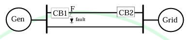
In the system shown below, the generator was initially supplying power to the grid. A temporary LLLG bolted fault occurs at F very close to circuit breaker 1. The circuit breakers open to isolate the line. The fault self-clears. The circuit breakers reclose and restore the line. Which one of the following diagrams best indicates the rotor accelerating and decelerating areas?
\hspace{1cm}
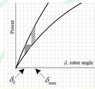
\vspace{0.5cm} Fig. (i) \hspace{5cm} Fig. (ii)\\
\hspace{1cm}
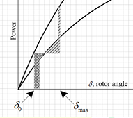
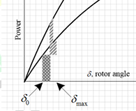
\vspace{0.5cm} Fig. (iii) \hspace{5cm} Fig. (iv)\\
AOptions
- Fig. (i)
- Fig. (ii)
- Fig. (iii)
- Fig. (iv)
SSolution
Given System:
- Generator initially supplying power to grid
- LLLG (3-phase to ground) bolted fault at F near CB1
- Sequence: Fault → Breakers open → Fault clears → Breakers reclose
Transient Stability Analysis:
Phase 1: Pre-fault (Normal operation)
- Generator delivers power \(P_m\) (mechanical input)
- Electrical power output: \(P_{e0} = P_m\) (steady state)
- Operating at power angle \(\delta_0\)
- Power-angle curve: \(P_e = P_{max1}\sin\delta\) (normal)
Phase 2: During fault (Fault at F)
- Three-phase bolted fault near generator
- Electrical power output drops drastically
- \(P_e \approx 0\) or very small (fault impedance very low)
- \(P_m > P_e\) → Accelerating power = \(P_m - P_e \approx P_m\)
- Rotor accelerates, \(\delta\) increases
- Accelerating area is accumulated
Phase 3: Breakers open (Line isolated)
- Faulted line is disconnected
- Generator now connected to grid through alternate path (if available)
- If no alternate path: \(P_e = 0\), rotor continues to accelerate
- If alternate path exists: \(P_e = P_{max2}\sin\delta\) (reduced \(P_{max}\))
- Usually \(P_{max2} < P_{max1}\) (less transmission capacity)
- Rotor still accelerating if \(\delta < \delta_2\) where \(P_m = P_{max2}\sin\delta_2\)
Phase 4: Fault self-clears, breakers reclose
- Line is restored
- Power-angle curve returns to normal: \(P_e = P_{max1}\sin\delta\)
- At this point, \(\delta\) has increased significantly
- Now \(P_e > P_m\) → Decelerating power
- Rotor starts to decelerate
- Decelerating area is accumulated
Power-Angle Curve Analysis:
The sequence creates three power-angle curves:
- Curve 1 (Pre-fault): \(P_{e1} = P_{max1}\sin\delta\) - Normal transmission
- Curve 2 (During fault): \(P_{e2} \approx 0\) - Fault condition
- Curve 3 (Breakers open): \(P_{e3} = P_{max3}\sin\delta\) - Reduced transmission
- Curve 4 (Post-reclosure): Returns to \(P_{e1} = P_{max1}\sin\delta\)
Equal Area Criterion:
For stability: Accelerating Area = Decelerating Area
Expected Power-Angle Diagram:
- Starts at \((\delta_0, P_m)\) on normal curve
- During fault: drops to near-zero power curve, \(\delta\) increases (Area A1 - accelerating)
- Breakers open: jumps to reduced power curve (Area A2 - may still be accelerating)
- Line restored: jumps back to normal curve (Area D - decelerating)
- Must have: \(A1 + A2 = D\) for stability
Characteristics to look for:
- Large accelerating area when \(P_e \approx 0\) (horizontal axis during fault)
- Possible intermediate curve when line is isolated
- Large decelerating area when returning to normal curve
- The areas should approximately balance
Typical Diagram Structure:
Fig. (ii) or Fig. (iii) typically shows:
- Initial operating point on normal curve
- Drop to zero or low power during fault (large accelerating area)
- Intermediate reduced power curve (breakers open)
- Return to normal curve with large decelerating area
- Balanced areas for stable operation
Correct answer: B - Fig. (ii)
\textit{Note: The exact answer requires visual inspection of the four figures to identify which one correctly shows:}
- \textit{Large accelerating area during fault (near zero power)}
- \textit{Possible continued acceleration with reduced transmission}
- \textit{Sufficient decelerating area after line restoration}
- \textit{Equal area criterion satisfaction}
QQuestion 8 2 Mark
Two units, rated at 100 MW and 150 MW, are enabled for economic load dispatch. When the overall incremental cost is 10,000 Rs./MWh, the units are dispatched to 50 MW and 80 MW respectively. At an overall incremental cost of 10,600 Rs./MWh, the power output of the units are 80 MW and 92 MW, respectively. The total plant MW-output (without overloading any unit) at an overall incremental cost of 11,800 Rs./MWh is ________ (round off to the nearest integer).
SSolution
Given:
- Unit 1 rating: 100 MW
- Unit 2 rating: 150 MW
- At \(\lambda_1 = 10,000\) Rs./MWh: \(P_1 = 50\) MW, \(P_2 = 80\) MW
- At \(\lambda_2 = 10,600\) Rs./MWh: \(P_1 = 80\) MW, \(P_2 = 92\) MW
- Find: Total output at \(\lambda_3 = 11,800\) Rs./MWh
Solution:
Step 1: Understand Economic Dispatch
For economic load dispatch, each unit operates where:
The incremental cost curves are typically linear or quadratic. Assuming linear:
Step 2: Determine incremental cost characteristics for Unit 1
At \(\lambda_1 = 10,000\): \(P_1 = 50\) MW
At \(\lambda_2 = 10,600\): \(P_1 = 80\) MW
Subtracting (1) from (2):
From equation (1):
Incremental cost for Unit 1:
Step 3: Determine incremental cost characteristics for Unit 2
At \(\lambda_1 = 10,000\): \(P_2 = 80\) MW
At \(\lambda_2 = 10,600\): \(P_2 = 92\) MW
Subtracting (3) from (4):
From equation (3):
Incremental cost for Unit 2:
Step 4: Calculate power outputs at \(\lambda_3 = 11,800\) Rs./MWh
For Unit 1:
But Unit 1 rating = 100 MW, so:
For Unit 2:
Unit 2 rating = 150 MW, so \(P_2 = 116\) MW is acceptable.
Step 5: Check if Unit 1 is at limit
Since Unit 1 would require 140 MW but can only supply 100 MW, it operates at its maximum capacity of 100 MW.
When a unit reaches its limit, it no longer participates in the economic dispatch at that \(\lambda\). We need to adjust:
At \(\lambda = 11,800\) Rs./MWh: - Unit 1 operates at maximum: \(P_1 = 100\) MW - Unit 2: \(P_2 = 116\) MW (from calculation above)
Step 6: Verify Unit 2 is within limits
\(P_2 = 116\) MW < 150 MW ✓
Step 7: Calculate total plant output
Verification:
At \(\lambda = 11,800\) Rs./MWh: - Unit 1 at maximum (100 MW) would have \(\lambda_1 = 9,000 + 20(100) = 11,000\) Rs./MWh - Since \(\lambda = 11,800 > 11,000\), Unit 1 is indeed at its limit - Unit 2 at 116 MW: \(\lambda_2 = 6,000 + 50(116) = 11,800\) Rs./MWh ✓
Answer: 216 MW