GATE 2024 Electrical Engineering (EE) Power Systems (2024)

Section 01

1-Mark Questions

QQuestion 1 1 Mark

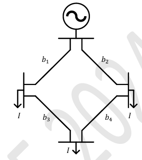
The figure shows the single line diagram of a 4-bus power network. Branches $b_1$, $b_2$, $b_3$, and $b_4$ have impedances $4z$, $z$, $2z$, and $4z$ per-unit (pu), respectively, where $z = r + jx$, with $r > 0$ and $x > 0$. The current drawn from each load bus (marked as arrows) is equal to $I$ pu, where $I \neq 0$. If the network is to operate with minimum loss, the branch that should be opened is

AOptions

$b_1$
$b_2$
$b_3$
$b_4$

SSolution

Given:

4-bus radial network with mesh
Branch impedances: $Z_{b1} = 4z$, $Z_{b2} = z$, $Z_{b3} = 2z$, $Z_{b4} = 4z$
Base impedance: $z = r + jx$ where $r > 0$, $x > 0$
Load current at each load bus: $I$ pu
Find: Which branch to open for minimum loss

Solution:

Step 1: Read the network

The generator bus at the top feeds $b_1$ to the left bus and $b_2$ to the right bus. The bottom bus is reached from the left bus through $b_3$ and from the right bus through $b_4$, closing one loop. The left, right and bottom buses each draw $I$ pu.

Step 2: With one branch open the currents are fixed by inspection

Opening a branch makes the network radial, so each remaining branch carries exactly the loads downstream of it and

\[P_{loss} = \sum_k |I_k|^2 R_k\]

can be evaluated exactly in each case. Below the currents are in units of $|I|$, the resistances in units of $r$, and the loss in units of $|I|^2 r$.

Open $b_1$: the left bus must be fed the long way, source $\to b_2 \to b_4 \to b_3$, so $b_2$ carries $3I$, $b_4$ carries $2I$ and $b_3$ carries $I$.

\[P_{loss} = 3^2(1) + 2^2(4) + 1^2(2) = 9 + 16 + 2 = 27\]

Open $b_2$: the right bus is fed through $b_1 \to b_3 \to b_4$, so $b_1$ carries $3I$, $b_3$ carries $2I$ and $b_4$ carries $I$.

\[P_{loss} = 3^2(4) + 2^2(2) + 1^2(4) = 36 + 8 + 4 = 48\]

Open $b_3$: $b_1$ feeds the left bus alone, $b_2$ feeds the right and bottom buses, $b_4$ feeds the bottom bus.

\[P_{loss} = 1^2(4) + 2^2(1) + 1^2(4) = 4 + 4 + 4 = 12\]

Open $b_4$: $b_1$ feeds the left and bottom buses, $b_3$ feeds the bottom bus, $b_2$ feeds the right bus.

\[P_{loss} = 2^2(4) + 1^2(2) + 1^2(1) = 16 + 2 + 1 = 19\]

Step 3: Compare

The four losses are 27, 48, 12 and 19 units. The smallest is obtained by opening $b_3$: that is the only arrangement in which the doubled current $2I$ is carried by $b_2$, the branch of least resistance $r$, while the two $4z$ branches each carry only $I$.

Note that the rule "open the highest-impedance branch" fails here, because the loss depends on $I^2 R$ and opening $b_1$ or $b_4$ forces large currents through other branches.

Correct answer: C ($b_3$)

QQuestion 2 1 Mark

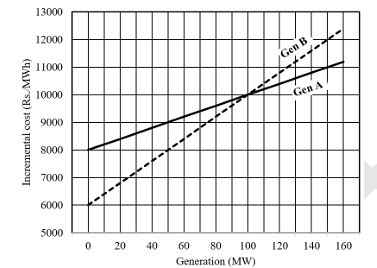
The incremental cost curves of two generators (Gen A and Gen B) in a plant supplying a common load are shown in the figure. If the incremental cost of supplying the common load is Rs. 7400 per MWh, then the common load in MW is _______ (rounded off to the nearest integer).

SSolution

Given:

Two generators: Gen A and Gen B
Incremental cost curves provided (graph)
System incremental cost: $\lambda = 7400$ Rs./MWh
Find: Total load (MW)

Solution:

Step 1: Understanding economic dispatch

For economic load dispatch, both generators operate at the same incremental cost:

\[\frac{dC_A}{dP_A} = \frac{dC_B}{dP_B} = \lambda\]

where $\lambda$ is the system incremental cost.

Step 2: Read the two characteristics off the graph

Both curves are straight lines and they cross at 100 MW, 10000 Rs./MWh:

Gen A passes through (0 MW, 8000) and (100 MW, 10000), so $\lambda_A = 8000 + 20 P_A$.
Gen B passes through (0 MW, 6000) and (100 MW, 10000), so $\lambda_B = 6000 + 40 P_B$.

Step 3: Apply $\lambda = 7400$ Rs./MWh

For Gen A:

\[8000 + 20 P_A = 7400 \Rightarrow P_A = -30 \text{ MW}\]

which is not feasible. The horizontal line at 7400 Rs./MWh lies below Gen A's incremental cost even at zero output, so Gen A does not run and $P_A = 0$.

For Gen B:

\[6000 + 40 P_B = 7400 \Rightarrow P_B = \frac{1400}{40} = 35 \text{ MW}\]

Step 4: Common load

\[P_{total} = P_A + P_B = 0 + 35 = 35 \text{ MW}\]

The 7400 Rs./MWh line cuts only the Gen B characteristic, which is why the whole load is carried by Gen B.

Answer: 35 MW

Section 02

2-Mark Questions

QQuestion 3 2 Mark

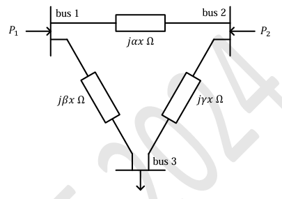
For the three-bus lossless power network shown in the figure, the voltage magnitudes at all the buses are equal to 1 per unit (pu), and the differences of the voltage phase angles are very small. The line reactances are marked in the figure, where $\alpha$, $\beta$, $\gamma$, and $x$ are strictly positive. The bus injections $P_1$ and $P_2$ are in pu. If $P_1 = mP_2$, where $m > 0$, and the real power flow from bus 1 to bus 2 is 0 pu, then which one of the following options is correct?

AOptions

$\gamma = m\beta$
$\beta = m\gamma$
$\alpha = m\gamma$
$\alpha = m\beta$

SSolution

Given:

Three-bus lossless network
Voltage magnitudes: $|V_1| = |V_2| = |V_3| = 1$ pu
Phase angle differences are very small
Line reactances: $j\alpha x$, $j\beta x$, $j\gamma x$
Bus injections: $P_1 = mP_2$ where $m > 0$
Power flow from bus 1 to bus 2: $P_{12} = 0$
Find: Relationship between $\alpha$, $\beta$, $\gamma$, and $m$

Solution:

Step 1: Power flow equations for small angle differences

For small angle differences and $|V| = 1$ pu:

Power flow from bus $i$ to bus $j$:

\[P_{ij} = \frac{V_i V_j}{X_{ij}}\sin(\delta_i - \delta_j) \approx \frac{\delta_i - \delta_j}{X_{ij}}\]

where the approximation $\sin(\delta_i - \delta_j) \approx \delta_i - \delta_j$ holds for small angles.

Step 2: Define power flows

Let:

$\delta_1$, $\delta_2$, $\delta_3$ = voltage angles at buses 1, 2, 3
$P_{12}$ = power flow from bus 1 to bus 2 (through reactance $j\alpha x$)
$P_{13}$ = power flow from bus 1 to bus 3 (through reactance $j\beta x$)
$P_{23}$ = power flow from bus 2 to bus 3 (through reactance $j\gamma x$)

Power flows:

\[P_{12} = \frac{\delta_1 - \delta_2}{\alpha x}\]

\[P_{13} = \frac{\delta_1 - \delta_3}{\beta x}\]

\[P_{23} = \frac{\delta_2 - \delta_3}{\gamma x}\]

Step 3: Apply power balance at buses

At bus 1:

\[P_1 = P_{12} + P_{13}\]

At bus 2:

\[P_2 = P_{23} - P_{12}\]

(Power injected = Power flowing out - Power flowing in)

At bus 3:

\[-(P_1 + P_2) = -P_{13} - P_{23}\]

\textbf{Step 4: Apply given condition $P_{12} = 0$}

From $P_{12} = 0$:

\[\frac{\delta_1 - \delta_2}{\alpha x} = 0\]

\[\delta_1 = \delta_2\]

Step 5: Express power injections

With $\delta_1 = \delta_2$:

At bus 1:

\[P_1 = 0 + P_{13} = \frac{\delta_1 - \delta_3}{\beta x}\]

\[P_1 = \frac{\delta_1 - \delta_3}{\beta x}\]

At bus 2:

\[P_2 = P_{23} - 0 = \frac{\delta_2 - \delta_3}{\gamma x}\]

Since $\delta_1 = \delta_2$:

\[P_2 = \frac{\delta_1 - \delta_3}{\gamma x}\]

Step 6: Apply condition $P_1 = mP_2$

\[\frac{\delta_1 - \delta_3}{\beta x} = m \times \frac{\delta_1 - \delta_3}{\gamma x}\]

Assuming $\delta_1 \neq \delta_3$ (otherwise no power flow):

\[\frac{1}{\beta x} = \frac{m}{\gamma x}\]

\[\frac{1}{\beta} = \frac{m}{\gamma}\]

\[\gamma = m\beta\]

Verification:

The relationship $\gamma = m\beta$ ensures that when:

Bus 1 and bus 2 are at the same angle ($\delta_1 = \delta_2$)
Both inject power to bus 3
Power injection ratio is $P_1/P_2 = m$
Line reactances satisfy $\gamma = m\beta$

This creates a balanced power distribution where no power flows between buses 1 and 2.

Physical interpretation:

Buses 1 and 2 act as a common generation point (same angle)
Both supply bus 3 (load or lower voltage bus)
The reactance ratio determines how power divides
To have $P_1 = mP_2$ with $P_{12} = 0$, we need $\gamma = m\beta$

Correct answer: A ($\gamma = m\beta$)

QQuestion 4 2 Mark

For a two-phase network, the phase voltages $V_p$ and $V_q$ are to be expressed in terms of sequence voltages $V_\alpha$ and $V_\beta$ as $\begin{bmatrix} V_p \\ V_q \end{bmatrix} = \mathbf{S} \begin{bmatrix} V_\alpha \\ V_\beta \end{bmatrix}$. The possible option(s) for matrix $\mathbf{S}$ is/are

AOptions

$\begin{bmatrix} 1 & 1 \\ 1 & -1 \end{bmatrix}$
$\begin{bmatrix} 1 & 1 \\ 1 & 1 \end{bmatrix}$
$\begin{bmatrix} 1 & 1 \\ 1 & 0 \end{bmatrix}$
$\begin{bmatrix} -1 & 1 \\ 1 & 1 \end{bmatrix}$

SSolution

Understanding Sequence Components:

Concept: Sequence components decompose an unbalanced system into balanced (symmetrical) components.

For a two-phase system:

Phase voltages: $V_p$ and $V_q$
Sequence voltages: $V_\alpha$ (positive sequence) and $V_\beta$ (negative sequence)

General transformation:

\[\begin{bmatrix} V_p \\ V_q \end{bmatrix} = \mathbf{S} \begin{bmatrix} V_\alpha \\ V_\beta \end{bmatrix}\]

\textbf{Requirements for valid transformation matrix $\mathbf{S}$:}

1. Linear independence: The matrix $\mathbf{S}$ must be non-singular (invertible):

\[\det(\mathbf{S}) \neq 0\]

This ensures unique mapping between phase and sequence domains.

2. Symmetrical columns: each column of $\mathbf{S}$ must itself be a balanced set for the two-phase system. For an $n$-phase system the sequence operator is $a = e^{j2\pi/n}$; with $n = 2$ this gives $a = -1$, so the only admissible column patterns are

\[\begin{bmatrix} 1 \\ 1 \end{bmatrix} \text{ (in phase)} \qquad \text{and} \qquad \begin{bmatrix} 1 \\ -1 \end{bmatrix} \text{ (anti-phase)}\]

each to within a non-zero scale factor, and the two columns may be interchanged. Invertibility alone is not sufficient.

Analysis of each option:

\textbf{Option (A): $\mathbf{S} = \begin{bmatrix} 1 & 1 \\ 1 & -1 \end{bmatrix}$}

Determinant:

\[\det(\mathbf{S}) = (1)(-1) - (1)(1) = -1 - 1 = -2 \neq 0$$ ✓ Physical meaning: $$V_p = V_\alpha + V_\beta\]

\[V_q = V_\alpha - V_\beta\]

This is valid. It represents:

$V_\alpha = \frac{V_p + V_q}{2}$ (average/common mode)
$V_\beta = \frac{V_p - V_q}{2}$ (difference/differential mode)

Option (A) is correct ✓

\textbf{Option (B): $\mathbf{S} = \begin{bmatrix} 1 & 1 \\ 1 & 1 \end{bmatrix}$}

Determinant:

\[\det(\mathbf{S}) = (1)(1) - (1)(1) = 0$$ ✗ Matrix is singular (not invertible). Cannot uniquely transform back to sequence components. $$V_p = V_\alpha + V_\beta\]

\[V_q = V_\alpha + V_\beta\]

This gives $V_p = V_q$ always, losing one degree of freedom.

Option (B) is incorrect ✗

\textbf{Option (C): $\mathbf{S} = \begin{bmatrix} 1 & 1 \\ 1 & 0 \end{bmatrix}$}

Determinant:

\[\det(\mathbf{S}) = (1)(0) - (1)(1) = -1 \neq 0$$ ✓ Physical meaning: $$V_p = V_\alpha + V_\beta\]

\[V_q = V_\alpha\]

The matrix is invertible, but its second column is $\begin{bmatrix} 1 \\ 0 \end{bmatrix}$: a component that appears on phase $p$ and is absent from phase $q$. That is not a balanced two-phase set, so $V_\alpha$ and $V_\beta$ defined this way are not sequence quantities, only an arbitrary invertible change of variables.

Option (C) is incorrect ✗

\textbf{Option (D): $\mathbf{S} = \begin{bmatrix} -1 & 1 \\ 1 & 1 \end{bmatrix}$}

Determinant:

\[\det(\mathbf{S}) = (-1)(1) - (1)(1) = -1 - 1 = -2 \neq 0$$ ✓ Physical meaning: $$V_p = -V_\alpha + V_\beta\]

\[V_q = V_\alpha + V_\beta\]

The columns are $\begin{bmatrix} -1 \\ 1 \end{bmatrix} = -\begin{bmatrix} 1 \\ -1 \end{bmatrix}$ and $\begin{bmatrix} 1 \\ 1 \end{bmatrix}$, i.e. the anti-phase and in-phase sets with the roles of $V_\alpha$ and $V_\beta$ interchanged and one sign reversed. Both columns are balanced sets, so this is a valid sequence transformation, with

$V_\alpha = \frac{V_q - V_p}{2}$
$V_\beta = \frac{V_p + V_q}{2}$

Option (D) is correct ✓

Summary:

A valid sequence transformation must be

non-singular, $\det(\mathbf{S}) \neq 0$, and
built from balanced two-phase columns, $\begin{bmatrix} 1 \\ 1 \end{bmatrix}$ and $\begin{bmatrix} 1 \\ -1 \end{bmatrix}$, up to scaling, sign and interchange.

(A) and (D) satisfy both. (B) is singular. (C) is invertible but one of its columns is not a balanced set, so it is not a sequence transformation.

Correct answers: A and D

QQuestion 5 2 Mark

Which of the following options is/are correct for the Automatic Generation Control (AGC) and Automatic Voltage Regulator (AVR) installed with synchronous generators?

AOptions

AGC response has a local effect on frequency while AVR response has a global effect on voltage.
AGC response has a global effect on frequency while AVR response has a local effect on voltage.
AGC regulates the field current of the synchronous generator while AVR regulates the generator's mechanical power input.
AGC regulates the generator's mechanical power input while AVR regulates the field current of the synchronous generator.

SSolution

Understanding AGC and AVR:

Automatic Generation Control (AGC):

Controls active power (P) output of generator
Regulates system frequency
Acts on prime mover (turbine governor)
Changes mechanical power input to generator

Automatic Voltage Regulator (AVR):

Controls reactive power (Q) output
Regulates generator terminal voltage
Acts on excitation system
Changes field current of generator

Analysis of Options:

Option (A): AGC → local frequency effect; AVR → global voltage effect

Analysis:

Frequency is a system-wide parameter
All synchronous machines in an interconnected system operate at the same frequency
Change in generation at one location affects frequency everywhere
Therefore: AGC has global effect on frequency ✗

Voltage is a localized parameter
Voltage varies from bus to bus
AVR primarily affects voltage at and near the generator terminal
Distant buses are less affected
Therefore: AVR has local effect on voltage ✗

Option (A) is incorrect ✗

Option (B): AGC → global frequency effect; AVR → local voltage effect

Analysis:

AGC and Frequency:

Frequency depends on system-wide active power balance
$\Delta f \propto \Delta P$ (frequency deviation proportional to power imbalance)
All generators in synchronous operation share the same frequency
AGC action at any generator affects entire system frequency
Global effect ✓

AVR and Voltage:

Voltage profile varies spatially across the network
Changing excitation affects primarily the local bus and nearby buses
Remote buses experience minimal voltage change
Voltage drop along transmission lines limits the range of influence
Local effect ✓

Option (B) is correct ✓

Option (C): AGC → field current; AVR → mechanical power

This is exactly opposite to the actual functions:

AGC controls mechanical power (governor) ✗
AVR controls field current (exciter) ✗

Option (C) is incorrect ✗

Option (D): AGC → mechanical power; AVR → field current

AGC Operation:

Measures system frequency
Compares with reference (usually 50 or 60 Hz)
Sends signal to turbine governor
Adjusts steam/water/fuel flow to prime mover
Changes mechanical power input: $P_m$
Regulates mechanical power ✓

AVR Operation:

Measures generator terminal voltage
Compares with reference voltage
Sends signal to excitation system
Adjusts DC excitation to field winding
Changes field current: $I_f$
Changes field flux: $\phi \propto I_f$
Regulates field current ✓

Option (D) is correct ✓

Summary of Control Actions:

\begin{tabular}{|l|l|l|} \hline Control & Regulates & Effect \\ \hline AGC & Mechanical power $P_m$ & Global (frequency) \\ AVR & Field current $I_f$ & Local (voltage) \\ \hline \end{tabular}

Physical Principles:

Why frequency effect is global:

All synchronous machines are electromagnetically coupled
Rotor speeds are synchronized
$f = \frac{P \cdot N_s}{120}$ where $N_s$ is synchronous speed
System operates at single frequency
Power imbalance anywhere affects frequency everywhere

Why voltage effect is local:

Voltage determined by Ohm's law: $V = IZ$
Impedance of transmission lines causes voltage drop
Reactive power flow strongly affects local voltage
Limited transmission of reactive power over long distances
Each bus can have different voltage magnitude

Correct answers: B and D

\textit{Note: This is a fundamental concept in power system control. AGC maintains system frequency (global parameter) by controlling active power, while AVR maintains terminal voltage (local parameter) by controlling excitation/field current.}

QQuestion 6 2 Mark

In the circuit shown, $Z_1 = 50\angle -90°$ $\Omega$ and $Z_2 = 200\angle -30°$ $\Omega$. It is supplied by a three phase 400 V source with the phase sequence being R-Y-B. Assume the wattmeters $W_1$ and $W_2$ to be ideal. The magnitude of the difference between the readings of $W_1$ and $W_2$ in watts is ___________ (rounded off to 2 decimal places).

SSolution

Given:

Three-phase supply: 400 V (line voltage), 50 Hz
Phase sequence: R-Y-B
Load impedances: $Z_1 = 50\angle -90°$ $\Omega$, $Z_2 = 200\angle -30°$ $\Omega$
Two wattmeters: $W_1$ and $W_2$ (ideal)
Find: $|W_1 - W_2|$ in watts

Solution:

Step 1: Analyze the impedances

$Z_1 = 50\angle -90° = 50(\cos(-90°) + j\sin(-90°)) = -j50 \text{ } \Omega$

This is purely capacitive: $Z_1 = -jX_C = -j50$ $\Omega$

$Z_2 = 200\angle -30° = 200(\cos(-30°) + j\sin(-30°))$ $Z_2 = 200(0.866 - j0.5) = 173.2 - j100 \text{ } \Omega$

Step 2: Read the connections from the figure

The two load branches meet on the R line: $Z_1$ is connected between R and B, $Z_2$ between R and Y.
$W_1$: current coil in line R, pressure coil across R-B.
$W_2$: current coil in line Y, pressure coil across Y-B.

Line B is the common line, so this is the standard two-wattmeter connection and $W_1 + W_2$ must equal the total active power.

Step 3: Line voltages (sequence R-Y-B)

\[V_{RY} = 400\angle 0°, \quad V_{YB} = 400\angle -120°, \quad V_{BR} = 400\angle 120° \text{ V}\]

\[V_{RB} = -V_{BR} = 400\angle -60° \text{ V}\]

Step 4: Branch and line currents

\[I_{Z1} = \frac{V_{RB}}{Z_1} = \frac{400\angle -60°}{50\angle -90°} = 8\angle 30° \text{ A}\]

\[I_{Z2} = \frac{V_{RY}}{Z_2} = \frac{400\angle 0°}{200\angle -30°} = 2\angle 30° \text{ A}\]

\[I_R = I_{Z1} + I_{Z2} = 10\angle 30° \text{ A}, \qquad I_Y = -I_{Z2} = 2\angle -150° \text{ A}\]

Step 5: Wattmeter readings

\[W_1 = |V_{RB}||I_R|\cos(\angle V_{RB} - \angle I_R) = 400 \times 10 \times \cos(-60° - 30°) = 4000\cos 90° = 0 \text{ W}\]

\[W_2 = |V_{YB}||I_Y|\cos(\angle V_{YB} - \angle I_Y) = 400 \times 2 \times \cos(-120° + 150°) = 800\cos 30° = 692.82 \text{ W}\]

Step 6: Difference of the readings

\[|W_1 - W_2| = |0 - 692.82| = 692.82 \text{ W}\]

Check: $W_1 + W_2 = 692.82$ W must be the total active power. $Z_1$ is purely capacitive and absorbs none, while $Z_2$ absorbs $|I_{Z2}|^2\operatorname{Re}(Z_2) = 2^2 \times 173.2 = 692.8$ W. $W_1$ reads zero because $I_R$ happens to lead $V_{RB}$ by exactly $90°$.

Answer: 692.82 W

QQuestion 7 2 Mark

Consider the closed-loop system shown in the figure with

$G(s) = \frac{K(s^2 - 2s + 2)}{(s^2 + 2s + 5)}$

The root locus for the closed-loop system is to be drawn for $0 \leq K < \infty$. The angle of departure (between 0° and 360°) of the root locus branch drawn from the pole $(-1 + j2)$, in degrees, is _________________ (rounded off to the nearest integer).

SSolution

Given:

Open-loop transfer function: $G(s) = \frac{K(s^2 - 2s + 2)}{(s^2 + 2s + 5)}$
Closed-loop system with unity feedback
Find: Angle of departure from pole at $s = -1 + j2$

Solution:

Step 1: Identify poles and zeros

Poles: Roots of $s^2 + 2s + 5 = 0$

$s = \frac{-2 \pm \sqrt{4 - 20}}{2} = \frac{-2 \pm \sqrt{-16}}{2} = \frac{-2 \pm j4}{2}$

$s = -1 \pm j2$

Poles: $p_1 = -1 + j2$ and $p_2 = -1 - j2$

Zeros: Roots of $s^2 - 2s + 2 = 0$

$s = \frac{2 \pm \sqrt{4 - 8}}{2} = \frac{2 \pm \sqrt{-4}}{2} = \frac{2 \pm j2}{2}$

$s = 1 \pm j1$

Zeros: $z_1 = 1 + j1$ and $z_2 = 1 - j1$

Step 2: Plot poles and zeros on s-plane

Pole $p_1$: $(-1, +2)$ - upper left quadrant
Pole $p_2$: $(-1, -2)$ - lower left quadrant
Zero $z_1$: $(1, +1)$ - upper right quadrant
Zero $z_2$: $(1, -1)$ - lower right quadrant

Step 3: Angle of departure formula

Applying the angle condition $\angle G(s) = 180°$ at a point just off the pole $p_1$ gives the angle of departure $\phi_d$:

$\phi_d = 180° + \sum \text{(angles from the zeros to } p_1) - \sum \text{(angles from the other poles to } p_1)$

Step 4: Calculate angles from zeros to $p_1 = -1 + j2$

From zero $z_1 = 1 + j1$ to $p_1 = -1 + j2$:

Vector: $p_1 - z_1 = (-1 + j2) - (1 + j1) = -2 + j1$

Angle: $\theta_{z1} = \tan^{-1}\left(\frac{1}{-2}\right) + 180°$ (in second quadrant)

$\theta_{z1} = \tan^{-1}(-0.5) + 180° = -26.57° + 180° = 153.43°$

From zero $z_2 = 1 - j1$ to $p_1 = -1 + j2$:

Vector: $p_1 - z_2 = (-1 + j2) - (1 - j1) = -2 + j3$

Angle: $\theta_{z2} = \tan^{-1}\left(\frac{3}{-2}\right) + 180°$ (in second quadrant)

$\theta_{z2} = \tan^{-1}(-1.5) + 180° = -56.31° + 180° = 123.69°$

Step 5: Calculate angle from other pole to $p_1$

From pole $p_2 = -1 - j2$ to $p_1 = -1 + j2$:

Vector: $p_1 - p_2 = (-1 + j2) - (-1 - j2) = j4$

Angle: $\theta_{p2} = 90°$ (positive imaginary axis)

Step 6: Apply the angle of departure formula

$\phi_d = 180° + \theta_{z1} + \theta_{z2} - \theta_{p2}$

$\phi_d = 180° + 153.43° + 123.69° - 90°$

$\phi_d = 367.12°$

Reducing to the range $0°$ to $360°$: $\phi_d = 367.12° - 360° = 7.12°$

Rounded to the nearest integer: $\phi_d = 7°$

Verification from the angle condition

Put $s = p_1 + \epsilon e^{j\phi_d}$ with $\epsilon \to 0$. The condition $\angle G(s) = 180°$ reads

$\angle(s - z_1) + \angle(s - z_2) - \angle(s - p_1) - \angle(s - p_2) = 180°$

$153.43° + 123.69° - \phi_d - 90° = 180°$

$\phi_d = 153.43° + 123.69° - 90° - 180° = 7.12°$

Answer: 7°

\textit{The branch leaves the pole at $-1 + j2$ almost horizontally, moving to the right and very slightly upward. That is consistent with the right-half-plane zeros at $1 \pm j1$, which draw the locus across the imaginary axis as $K$ increases.}