GATE 2015 Electrical Engineering (EE) Power Systems (2015)

Section 01

1-Mark Questions

QQuestion 1 1 Mark

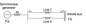
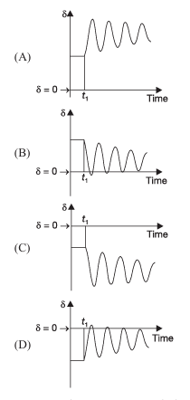
Q46 (Set-1): Synchronous generator supplying infinite bus via two parallel lines, one trips at \(t_1\). Which waveform shows rotor angle \(\delta\) transient correctly?

SSolution

Transient analysis:

Before trip: System stable at operating angle \(\delta_0\)

At \(t_1\): One line trips

System reactance increases
Power transfer capability reduces
If \(P_m >\) new \(P_{max}\sin\delta_0\), rotor accelerates
\(\delta\) increases

Stable transient characteristics:

\(\delta\) increases beyond initial value
Oscillates around new equilibrium
Eventually settles (with damping)
Maximum swing < critical angle

Before the trip the machine delivers power to the bus, so \(\delta_0 > 0\). Removing Line 1 raises the transfer reactance and lowers \(P_{max}\); with \(P_m\) unchanged the new equilibrium satisfies \(\sin\delta_{new} > \sin\delta_0\). The rotor angle therefore rises from a positive \(\delta_0\) to a larger positive value and swings about it with decaying amplitude.

Only waveform (A) shows this. (B) has \(\delta\) falling after \(t_1\), and (C) and (D) start from a negative \(\delta_0\).

Answer: A

QQuestion 2 1 Mark

Q47 (Set-1): 3-bus system with bus admittance matrix. If shunt capacitance of all lines 50% compensated, imaginary part of \(Y_{33}\) (in pu) after compensation is

AOptions

-j7.0
-j8.5
-j7.5
-j9.0

SSolution

Bus admittance element:

Original \(Y_{33} = -j8\) pu

This equals: \(Y_{33} = Y_{30} + Y_{31} + Y_{32}\)

Where \(Y_{30}\) is shunt admittance at bus 3.

From matrix:

\[-j8 = Y_{30} + (-j4) + (-j5)\]

\[Y_{30} = -j8 + j9 = j1\]

This represents shunt capacitive susceptance.

After 50% compensation:

Compensation reduces shunt capacitance by 50%:

\[Y_{30,new} = \frac{j1}{2} = j0.5\]

\textbf{New \(Y_{33}\):}

\[Y_{33,new} = j0.5 + (-j4) + (-j5)\]

\[= j0.5 - j9 = -j8.5\]

Answer: B

QQuestion 3 1 Mark

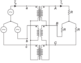
Q53 (Set-1): Star-Delta transformer, 230 V (line) star side, 115 V delta side. If \(I_s = 100\angle 0°\) A, value of \(I_p\) (in A) is

\subsection*{Set-2 Questions}

AOptions

\(50\angle 30°\)
\(50\angle -30°\)
\(50\sqrt{3}\angle 30°\)
\(200\angle 30°\)

SSolution

Power balance:

\[\sqrt{3}V_{L,p}I_p = \sqrt{3}V_{L,s}I_s\]

\[230I_p = 115 \times 100\]

\[I_p = \frac{11500}{230} = 50 \text{ A}\]

Phase relationship:

Star-Delta transformation introduces 30° phase shift.

Line current on star side leads corresponding line current on delta side by 30°.

\[I_p = 50\angle 30° \text{ A}\]

Answer: A

QQuestion 4 1 Mark

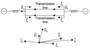
Q54 (Set-2): Sustained three-phase fault in power system. Current and voltage phasors shown. Where is fault located?

SSolution

Fault location analysis:

In the phasor diagram \(\bar{I}_2\) and \(\bar{I}_4\) are equal in magnitude and 180° apart. The lower circuit therefore carries only through-current — whatever enters one end leaves the other — so it is healthy and carries no fault infeed.

\(\bar{I}_1\) and \(\bar{I}_3\) both lag the bus voltages by roughly 90° and both feed into the upper circuit from opposite ends, so the fault lies on that line, between the two measuring points. \(|\bar{I}_1| > |\bar{I}_3|\), consistent with the stronger source seeing the shorter path to the fault.

Answer: B (Location Q)

Section 02

2-Mark Questions

QQuestion 5 2 Mark

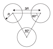
Q51 (Set-1): Composite conductor with 3 conductors of radius R in symmetrical spacing. GMR of composite (in cm) is \(kR\). Value of \(k\) is

SSolution

GMR of composite conductor:

For symmetrical spacing:

\[\text{GMR} = \sqrt[3]{\text{GMR}_1 \times \text{GMR}_2 \times \text{GMR}_3}\]

For each conductor:

\[\text{GMR}_i = 0.7788R\]

From the figure the three conductors sit at the corners of an equilateral triangle with centre-to-centre spacing \(d = 3R\).

The GMR of the composite is the 9th root of the nine distances from each strand to every strand:

\[\text{GMR} = \sqrt[9]{(r'\,d\,d)(d\,r'\,d)(d\,d\,r')} = \sqrt[9]{(r')^3 d^6} = (r')^{1/3} d^{2/3}\]

With \(r' = 0.7788R\) and \(d = 3R\):

\[\text{GMR} = (0.7788R)^{1/3}(3R)^{2/3} = (0.7788)^{1/3}(3)^{2/3}R = 0.9199 \times 2.0801 \times R\]

\[= 1.913R \;\Rightarrow\; k = 1.913\]

Answer: 1.85-1.95

QQuestion 6 2 Mark

Q51 (Set-2): Economic dispatch: \(C_1(P_1) = 0.01P_1^2 + 30P_1 + 10\) (100-150 MW); \(C_2(P_2) = 0.05P_2^2 + 10P_2 + 10\) (100-180 MW). For 200 MW load, incremental cost (in ₹/MWh) is

SSolution

Incremental costs:

\[\frac{dC_1}{dP_1} = 0.02P_1 + 30\]

\[\frac{dC_2}{dP_2} = 0.1P_2 + 10\]

Equal incremental cost:

\[0.02P_1 + 30 = 0.1P_2 + 10\]

With \(P_1 + P_2 = 200\):

\[0.02P_1 + 30 = 0.1(200 - P_1) + 10\]

\[0.02P_1 + 30 = 20 - 0.1P_1 + 10\]

\[0.12P_1 = 0\]

\[P_1 = 0\]

This violates minimum constraint.

At limits: \(P_1 = 100\) MW (minimum)

\[P_2 = 200 - 100 = 100 \text{ MW}\]

Incremental cost:

\[\frac{dC_2}{dP_2} = 0.1(100) + 10 = 20 \text{ ₹/MWh}\]

Answer: 20 ₹/MWh

QQuestion 7 2 Mark

Q53 (Set-2): 50 Hz generating unit, \(H = 2\) MJ/MVA. Initially \(\delta_0 = 5°\), \(P_m = 1\) pu. Three-phase fault at terminals. Value of \(\delta\) (in degrees) 0.02 s after fault is

SSolution

Swing equation:

\[\frac{d^2\delta}{dt^2} = \frac{\pi f_0}{H}(P_m - P_e)\]

During fault: \(P_e = 0\)

\[\frac{d^2\delta}{dt^2} = \frac{\pi \times 50}{2}(1 - 0) = 25\pi\]

Integration:

\[\frac{d\delta}{dt} = 25\pi t + C_1\]

At \(t = 0\): \(\frac{d\delta}{dt} = 0\) (initially steady)

\[C_1 = 0\]

\[\delta(t) = \frac{25\pi t^2}{2} + C_2\]

At \(t = 0\): \(\delta = 5° = 0.0873\) rad

\[C_2 = 0.0873\]

At \(t = 0.02\) s:

\[\delta = \frac{25\pi (0.02)^2}{2} + 0.0873\]

\[= \frac{25\pi \times 0.0004}{2} + 0.0873\]

\[= 0.0157 + 0.0873 = 0.103 \text{ rad}\]

\[= 5.9°\]

Answer: 5.90°

QQuestion 8 2 Mark

Q56 (Set-2): Two-port network: 10 V at Port 1 gives 4 A through short-circuited Port 2. 5 V at Port 1 gives 1.25 A through 1 \(\Omega\) at Port 2. For 3 V at Port 1 with 2 \(\Omega\) at Port 2, current (in A) is

SSolution

Let \(I\) be the current the network delivers into the load at port 2, and write the linear relation

\[I = aV_1 + bV_2\]

First test: \(V_1 = 10\) V, port 2 shorted so \(V_2 = 0\), \(I = 4\) A:

\[a = \frac{4}{10} = 0.4\]

Second test: \(V_1 = 5\) V, \(R_L = 1\ \Omega\), \(I = 1.25\) A, so \(V_2 = 1.25\) V:

\[1.25 = 0.4(5) + b(1.25) \;\Rightarrow\; b = -0.6\]

Third test: \(V_1 = 3\) V, \(R_L = 2\ \Omega\), so \(V_2 = 2I\):

\[I = 0.4(3) - 0.6(2I) = 1.2 - 1.2I\]

\[2.2I = 1.2 \;\Rightarrow\; I = 0.5454 \text{ A}\]

Answer: 0.5454 A