Introduction
-
Mathematical modeling of physical systems
-
Transfer function representation
-
Block diagram reduction techniques
-
Signal flow graphs (Mason’s Gain Formula)
-
Feedback concepts and properties
-
System types and error constants
Master the fundamentals of modeling and analyzing control systems with emphasis on problem-solving techniques for GATE EE examination.
Mathematical Modeling
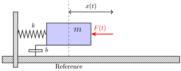
Mechanical Systems:
-
Mass (\(m\)): \(F = ma\)
-
Spring (\(k\)): \(F = kx\)
-
Damper (\(b\)): \(F = b\dot{x}\)
Electrical Systems:
-
Resistor (\(R\)): \(V = IR\)
-
Inductor (\(L\)): \(V = L\frac{dI}{dt}\)
-
Capacitor (\(C\)): \(I = C\frac{dV}{dt}\)
Mass-Spring-Damper System:
| Mechanical | Electrical | Relationship |
|---|---|---|
| Force \(F\) | Voltage \(V\) | Through variable |
| Velocity \(\dot{x}\) | Current \(I\) | Across variable |
| Mass \(m\) | Inductance \(L\) | \(F = m\ddot{x} \leftrightarrow V = L\frac{dI}{dt}\) |
| Damping \(b\) | Resistance \(R\) | \(F = b\dot{x} \leftrightarrow V = RI\) |
| Spring \(k\) | \(\frac{1}{C}\) | \(F = k\int \dot{x}dt \leftrightarrow V = \frac{1}{C}\int I dt\) |
Force-Current analogy is dual to Force-Voltage analogy. Choose the appropriate analogy based on the system configuration.
Transfer Function
The transfer function \(G(s)\) of a Linear Time-Invariant (LTI) system is defined as:
-
Valid only for LTI systems
-
Independent of input signal magnitude
-
Characteristic equation: \(1 + G(s)H(s) = 0\)
-
Poles: Roots of denominator polynomial
-
Zeros: Roots of numerator polynomial
-
System order = degree of denominator polynomial
For GATE problems, quickly identify system type by denominator degree:
-
Type 0: No \(s\) in denominator
-
Type 1: One \(s\) in denominator
-
Type 2: Two \(s\) terms in denominator
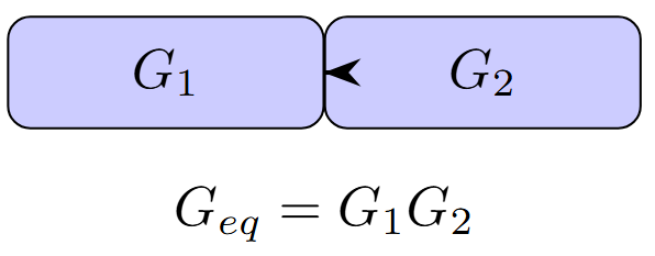
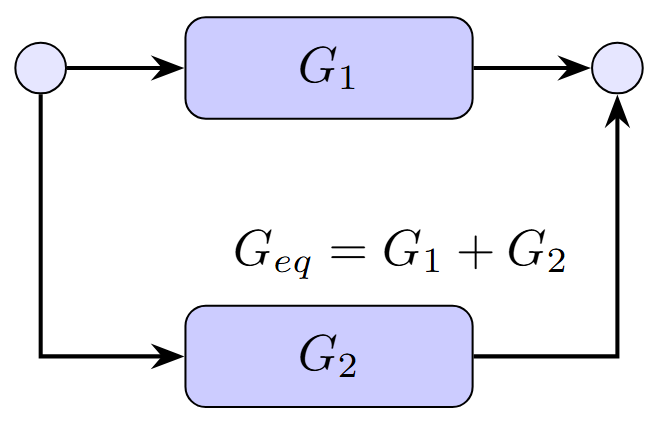
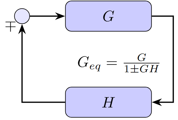
Block Diagrams
-
Negative feedback: \(\frac{G}{1 + GH}\)
-
Positive feedback: \(\frac{G}{1 - GH}\)
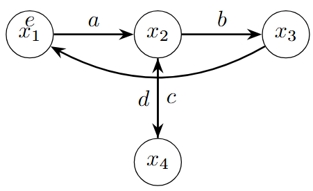
Signal Flow Graphs
-
Node: Junction point representing a variable
-
Branch: Directed line segment with gain
-
Path: Sequence of connected branches
-
Loop: Closed path
-
Forward Path: Path from input to output
-
Non-touching loops: Loops with no common nodes
The overall transfer function is:
-
\(P_k\) = Gain of \(k^{th}\) forward path
-
\(\Delta\) = Graph determinant
-
\(\Delta_k\) = Cofactor for \(k^{th}\) path
For complex systems, Mason’s formula is often faster than block diagram reduction.
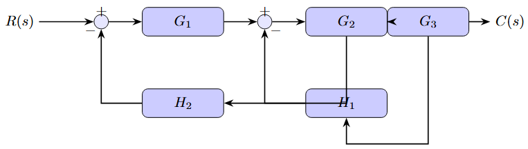
Consider the signal flow graph:
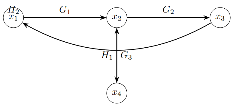
Solution:
-
Forward path: \(P_1 = G_1 G_2\)
-
Loops: \(L_1 = G_3 H_1\), \(L_2 = G_1 G_2 H_2\)
-
\(\Delta = 1 - (G_3 H_1 + G_1 G_2 H_2)\)
-
\(\Delta_1 = 1 - G_3 H_1\) (removing \(L_2\) which touches the forward path)
-
\(T = \frac{G_1 G_2 (1 - G_3 H_1)}{1 - G_3 H_1 - G_1 G_2 H_2}\)
Feedback Concepts
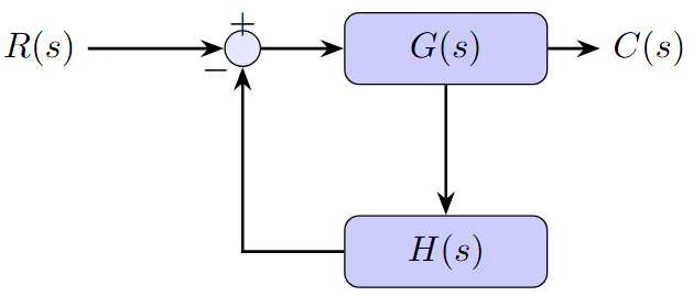
-
Error: \(E(s) = R(s) - H(s)C(s)\)
-
Closed-loop TF: \(T(s) = \frac{G(s)}{1 + G(s)H(s)}\)
-
Error TF: \(\frac{E(s)}{R(s)} = \frac{1}{1 + G(s)H(s)}\)
-
Open-loop TF: \(G(s)H(s)\)
-
Characteristic equation: \(1 + G(s)H(s) = 0\)
-
For unity feedback: \(H(s) = 1\)
-
Reduced sensitivity to parameter variations
-
Improved stability and transient response
-
Reduced effect of noise and disturbances
-
Improved accuracy in steady-state
-
Bandwidth modification possible
-
Reduced overall gain
-
Potential instability if poorly designed
-
Increased complexity and cost
-
May introduce noise through feedback path
Sensitivity of closed-loop system to open-loop gain variations:
System Types
Based on number of poles at origin in \(G(s)H(s)\):
-
Position Error Constant: \(K_p = \lim_{s \to 0} G(s)H(s)\)
-
Velocity Error Constant: \(K_v = \lim_{s \to 0} s \cdot G(s)H(s)\)
-
Acceleration Error Constant: \(K_a = \lim_{s \to 0} s^2 \cdot G(s)H(s)\)
-
Step input: \(e_{ss} = \frac{1}{1 + K_p}\)
-
Ramp input: \(e_{ss} = \frac{1}{K_v}\)
-
Parabolic input: \(e_{ss} = \frac{1}{K_a}\)
| System Type | \(K_p\) | \(K_v\) | \(K_a\) |
|---|---|---|---|
| Type 0 | \(K\) | \(0\) | \(0\) |
| Type 1 | \(\infty\) | \(K\) | \(0\) |
| Type 2 | \(\infty\) | \(\infty\) | \(K\) |
| Input | Type 0 | Type 1 | Type 2 |
|---|---|---|---|
| Step | \(\frac{1}{1+K_p}\) | \(0\) | \(0\) |
| Ramp | \(\infty\) | \(\frac{1}{K_v}\) | \(0\) |
| Parabolic | \(\infty\) | \(\infty\) | \(\frac{1}{K_a}\) |
GATE Practice
The transfer function of a system is \(G(s) = \frac{10}{s^2 + 3s + 2}\). The DC gain is:
-
0
-
5
-
10
-
\(\frac{10}{2} = 5\)
DC gain is found by substituting \(s = 0\):
For a unity feedback system with \(G(s) = \frac{4}{s(s+2)}\), the closed-loop transfer function is:
-
\(\frac{4}{s^2 + 2s + 4}\)
-
\(\frac{4}{s^2 + 2s}\)
-
\(\frac{2}{s^2 + 2s + 4}\)
-
\(\frac{4}{s + 2}\)
For unity feedback: \(H(s) = 1\)
A Type 1 system has \(G(s)H(s) = \frac{20}{s(s+4)}\). The velocity error constant \(K_v\) is:
-
4
-
5
-
20
-
\(\infty\)
For Type 1 system:
The Mason’s gain formula for the system shown requires calculation of:
-
Forward paths and loops only
-
Forward paths, loops, and their cofactors
-
Only the characteristic polynomial
-
Transfer function directly
Mason’s gain formula requires:
-
All forward paths and their gains
-
All loops and their gains
-
Cofactors for each forward path
-
Graph determinant calculation
Answer: B
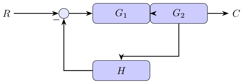
For the block diagram shown, if \(G_1 = 2\), \(G_2 = 3\), and \(H = 0.5\), the overall transfer function is:
-
\(\frac{6}{1+3}\)
-
\(\frac{6}{1+6}\)
-
\(\frac{6}{4}\)
-
\(\frac{2}{3}\)
A second-order system has the transfer function:
-
\(\omega_n = 5\) rad/s, \(\zeta = 0.4\)
-
\(\omega_n = 25\) rad/s, \(\zeta = 0.2\)
-
\(\omega_n = 5\) rad/s, \(\zeta = 0.2\)
-
\(\omega_n = 4\) rad/s, \(\zeta = 0.4\)
Standard form: \(G(s) = \frac{K\omega_n^2}{s^2 + 2\zeta\omega_n s + \omega_n^2}\)
Comparing: \(\omega_n^2 = 25 \Rightarrow \omega_n = 5\) rad/s
\(2\zeta\omega_n = 4 \Rightarrow \zeta = \frac{4}{2 \times 5} = 0.4\)
Answer: A
Summary
-
\(K_p = \lim_{s \to 0} G(s)H(s)\)
-
\(K_v = \lim_{s \to 0} s \cdot G(s)H(s)\)
-
\(K_a = \lim_{s \to 0} s^2 \cdot G(s)H(s)\)
-
Master block diagram reduction for complex systems
-
Understand Mason’s gain formula for signal flow graphs
-
Know system types and their error characteristics
-
Practice steady-state error calculations
-
Remember standard transfer function forms
-
Identify system type and structure
-
Choose appropriate analysis method (block diagram vs. Mason’s formula)
-
Apply reduction rules systematically
-
Verify results using alternative methods when possible
-
Check units and limiting cases