Electronic Devices & Circuits · Lecture 30

Active Filters

Analog Circuits & Applications

Dr. Mithun Mondal BITS Pilani, Hyderabad Campus

SECTION 01

Introduction

Introduction to Active Filters

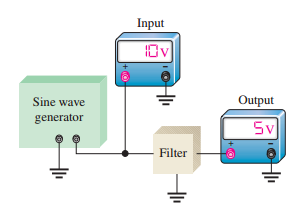
Filters process signals by passing selected frequencies while rejecting others
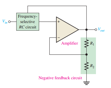
Active filters use op-amps with passive RC circuits
Filters categorized by output voltage variation with input frequency
Four basic categories:
- Low-pass
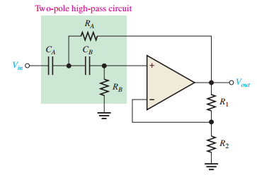
- High-pass
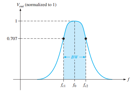
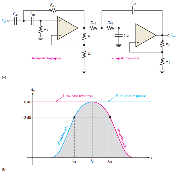
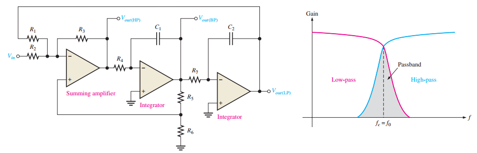
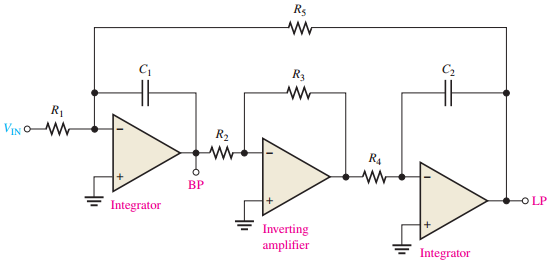
- Band-pass
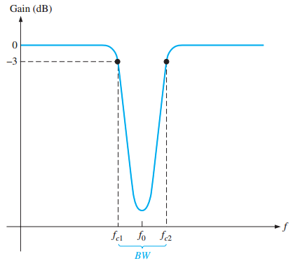
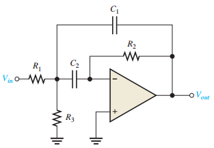
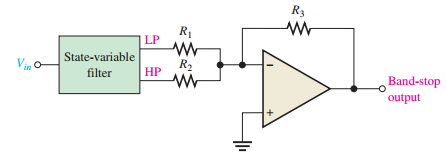
- Band-stop
Advantages over passive filters:
- Gain provided by active elements
- High input impedance
- Low output impedance

SECTION 02

Filter Responses

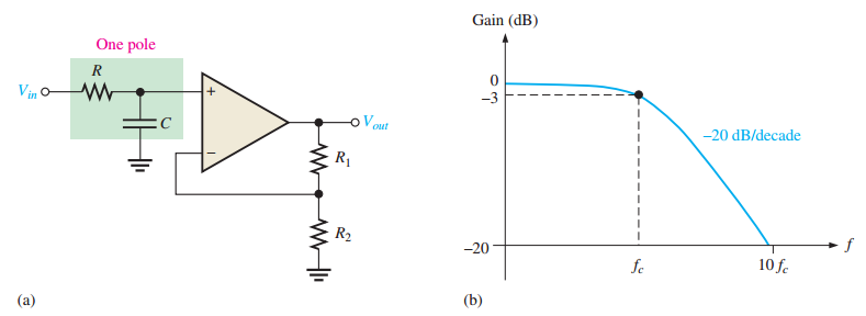
Low-Pass Filter Response

Passes frequencies from DC to critical frequency \(f_c\), attenuates others
Passband: Frequencies with \(< -3 \, \text{dB}\) attenuation
Critical frequency: \(f_c = \dfrac{1}{2 \pi R C}\) (single-pole \(RC\) filter)
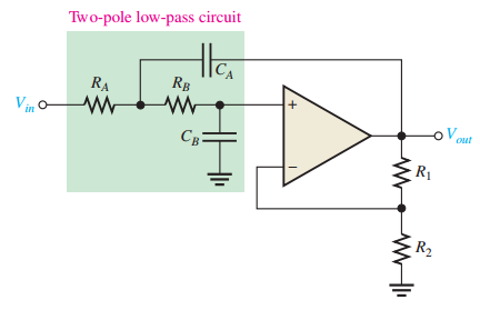
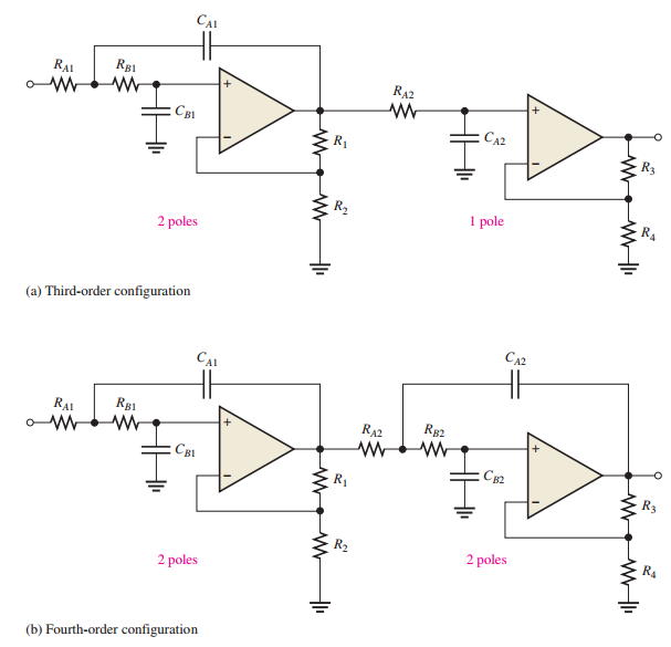
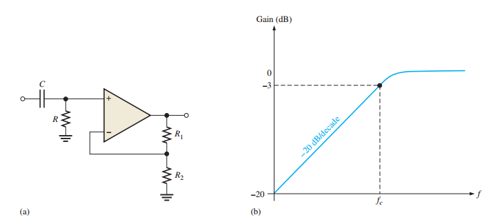
Roll-off: \(-20 \, \text{dB/decade}\) per pole
Bandwidth: \(BW = f_c\) (ideal)

High-Pass Filter Response

Passes frequencies above \(f_c\), attenuates below
Critical frequency: \(f_c = \dfrac{1}{2 \pi R C}\) (single-pole \(RC\) filter)
Roll-off: \(-20 \, \text{dB/decade}\) per pole
Practical limitation: Op-amp’s internal \(RC\) circuits limit high-frequency response

Band-Pass Filter Response

Passes frequencies between lower (\(f_{c1}\)) and upper (\(f_{c2}\)) critical frequencies
Bandwidth: \(BW = f_{c2} - f_{c1}\)
Center frequency: \(f_0 = \sqrt{f_{c1} f_{c2}}\)
Quality factor: \(Q = \dfrac{f_0}{BW} = \dfrac{1}{DF}\) (DF: Damping factor)
\(Q > 10\): Narrow-band; \(Q < 10\): Wide-band

Band-Stop Filter Response

Rejects frequencies between \(f_{c1}\) and \(f_{c2}\), passes others
Bandwidth: \(BW = f_{c2} - f_{c1}\)
Opposite of band-pass filter

SECTION 03

Filter Characteristics

Filter Response Characteristics

Butterworth: Flat passband, \(-20 \, \text{dB/decade/pole}\), nonlinear phase
Chebyshev: Steeper roll-off (\(> -20 \, \text{dB/decade/pole}\)), passband ripples
Bessel: Linear phase, minimal overshoot, suitable for pulse waveforms

Damping Factor

Determines response characteristic
Defined as: \(DF = 2 - \dfrac{R_1}{R_2}\)
Example: For second-order Butterworth, \(DF = 1.414\), so \(\dfrac{R_1}{R_2} = 0.586\)

Critical Frequency and Filter Order

Critical Frequency (\(f_c\)) for first-order RC filter: \[f_c = \frac{1}{2\pi RC}\]
Applies to both low-pass and high-pass single-pole configurations
Roll-Off Rate:
- Butterworth filter: \(-20\, \text{dB/decade/pole}\)
- 1st-order (1 pole): \(-20\, \text{dB/decade}\)
- 2nd-order (2 poles): \(-40\, \text{dB/decade}\)
- 3rd-order (3 poles): \(-60\, \text{dB/decade}\), etc.

SECTION 04

Filter Implementations

Single-Pole Low-Pass Filter

Uses one \(RC\) circuit, roll-off \(-20 \, \text{dB/decade}\)
Critical frequency: \(f_c = \dfrac{1}{2 \pi R C}\)
Gain: \(A_{cl(NI)} = \dfrac{R_1}{R_2} + 1\)

Sallen-Key Low-Pass Filter

Common second-order configuration (VCVS)
Two-pole filter, roll-off \(-40 \, \text{dB/decade}\)
Critical frequency: \(f_c = \dfrac{1}{2 \pi \sqrt{R_A R_B C_A C_B}}\)
If \(R_A = R_B = R\), \(C_A = C_B = C\): \(f_c = \dfrac{1}{2 \pi R C}\)

Cascaded Low-Pass Filters

Third-order: Cascade 2-pole Sallen-Key + 1-pole filter (\(-60 \, \text{dB/decade}\))
Fourth-order: Cascade two 2-pole Sallen-Key filters (\(-80 \, \text{dB/decade}\))

Single-Pole High-Pass Filter

Roll-off: \(-20 \, \text{dB/decade}\)
Critical frequency: \(f_c = \dfrac{1}{2 \pi R C}\)
Limitation: Op-amp’s internal \(RC\) limits high-frequency response

Sallen-Key High-Pass Filter

Two-pole filter, roll-off \(-40 \, \text{dB/decade}\)
\(R\) and \(C\) positions swapped compared to low-pass
Response optimized by feedback resistors \(R_1\), \(R_2\)

SECTION 05

Band-Pass and Band-Stop Filters

Cascaded Band-Pass Filter

Cascade high-pass and low-pass Sallen-Key filters
\(f_{c1} = \dfrac{1}{2 \pi \sqrt{R_{A1} R_{B1} C_{A1} C_{B1}}}\)
\(f_{c2} = \dfrac{1}{2 \pi \sqrt{R_{A2} R_{B2} C_{A2} C_{B2}}}\)
Center frequency: \(f_0 = \sqrt{f_{c1} f_{c2}}\)
Suitable for wide bandwidth applications

Multiple-Feedback Band-Pass Filter

Center frequency: \(f_0 = \dfrac{1}{2 \pi C \sqrt{\dfrac{R_1 + R_3}{R_1 R_2 R_3}}}\)
Gain: \(A_0 = \dfrac{R_2}{2 R_1}\)
Resistors:
- \(R_1 = \dfrac{Q}{2 \pi f_0 C A_0}\)
- \(R_2 = \dfrac{Q}{\pi f_0 C}\)
- \(R_3 = \dfrac{Q}{2 \pi f_0 C (2 Q^2 - A_0)}\)

State-Variable Filter

Uses summing amplifier and two integrators
Center frequency: \(f_0 \approx \dfrac{1}{2 \pi R C}\)
\(Q = \dfrac{1}{3} \left( \dfrac{R_5}{R_6} + 1 \right)\)
Provides low-pass, high-pass, band-pass outputs

Biquad Filter

Integrator, inverting amplifier, integrator
Provides band-pass and low-pass outputs
High \(Q\), bandwidth independent of \(f_0\)

Multiple-Feedback Band-Stop Filter

Similar to band-pass, with modified resistor configuration

State-Variable Band-Stop Filter

Created by summing LP and HP outputs
Common application: 60 Hz noise rejection
Center frequency set by integrator RC circuits

SECTION 06

Measurements

Filter Response Measurements

Discrete Point Measurement

Set constant input amplitude
Sweep frequency in steps
Record output at each frequency
Plot response curve

Swept Frequency Measurement

More efficient than discrete method
Uses swept frequency generator
Display options:
- Spectrum analyzer
- Oscilloscope in X-Y mode
Provides continuous response curve

SECTION 07

Summary

Covered low-pass, high-pass, band-pass, band-stop filters
Discussed Butterworth, Chebyshev, Bessel characteristics
Analyzed single-pole, Sallen-Key, multiple-feedback, state-variable, biquad filters
Explained damping factor, critical frequency, roll-off rates
Described discrete point and swept frequency measurements