Demonstrative Video
Equivalent Circuit
-
Practical transformer excluding no-load current:
-
\(R_i\) and \(X_i\) represents resistance and leakage reactance
-
-
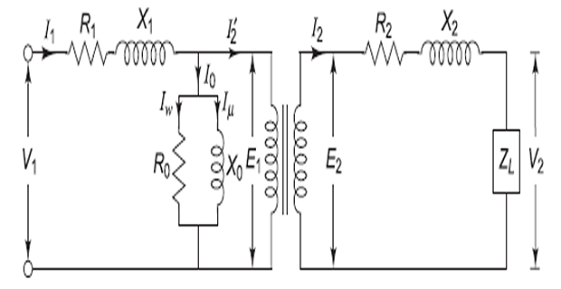
Practical transformer including no-load current components:
-
\(I_1 = I_0 + I_2^{\prime}\)
-
-
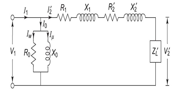
Modified Circuit of Primary Winding:
-
Note: Since all quantities are transferred to primary, the transformer need not be shown
-
As \(I_0\) is very small as compared to \(I_1~\Rightarrow\) drop across \(R_1\) and \(X_1\) due to \(I_0\) can be neglected \(\Rightarrow\) shift no-load components to the extreme left
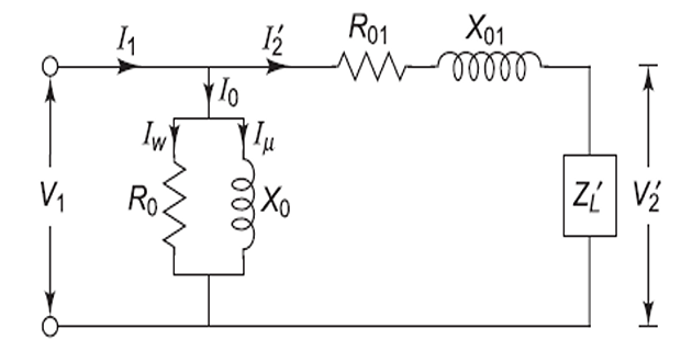
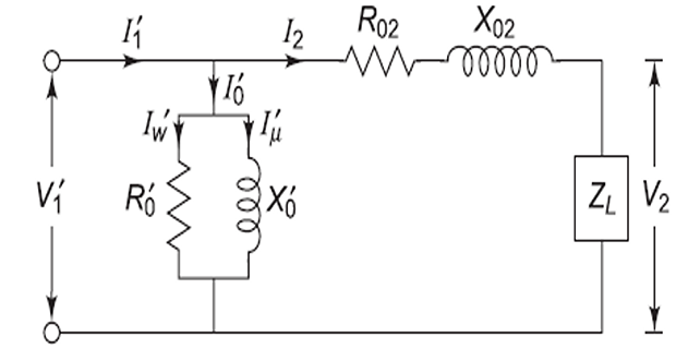
Equivalent parameters
referred to secondary:
Remember
-
Shifting primary R/X to the secondary, multiply it by \(K^2\)
-
Shifting secondary R/X to the primary, divide it \(K^2\)
Voltage Regulation
-
Transformer loaded, \(V_2~\downarrow\) due to a drop across \(R_2\) and \(X_2\) .
-
. from no load to full load conditions, expressed as a fraction of the no-load secondary voltage is called Change in\[\begin{aligned} \text{Regulation} & =\frac{\left(\begin{matrix}\text{Secondary terminal}\\ \text{voltage on no load}\end{matrix}\right)-\left(\begin{matrix}\text{Secondary terminal}\\ \text{voltage on full load}\end{matrix}\right)}{\text{Secondary terminal voltage on no load}}\\ & = \dfrac{E_2-V_2}{E_2} \\ \text{%Regulation} & = \dfrac{E_2-V_2}{E_2} \times 100 \end{aligned}\]
Efficiency
If \(x\) is the fraction of the full-load, then efficiency is given as
Condition for the maximum efficiency
-
\(V_2\) is constant
-
for a given \(\cos\Phi_2\) , \(\eta\) depends upon \(I_2\)
-
efficiency will be maximum when\[\begin{aligned} \dfrac{d}{dI_{2}} & =\left(V_{2}\cos\Phi_{2}+\dfrac{P_{i}}{I_{2}}+I_{2}R_{T}\right)=0\\ & \Rightarrow0-\dfrac{P_{i}}{I_{2}^{2}}+R_{T}=0\\ & \Rightarrow P_{i}=I_{2}^{2}R_{T}\\ & \boxed{\Rightarrow\mbox{Iron loss}=\mbox{copper loss}} \end{aligned}\]
OC & SC Tests
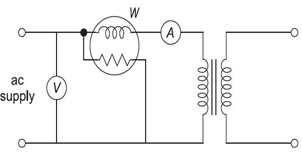
Open-Circuit Test (OC)
-
Purpose : To determine
-
iron loss or core loss ( \(W_i\) )
-
magnetising resistance ( \(R_0\) )
-
magnetising reactance ( \(X_0\) )
-
-
Test Connections :
-
HV open and supply and meters are connected to LV side
-
ammeter indicates no-load current (3-5% of F.L current)
-
Cu losses negligible and wattmeter indicates iron loss
-
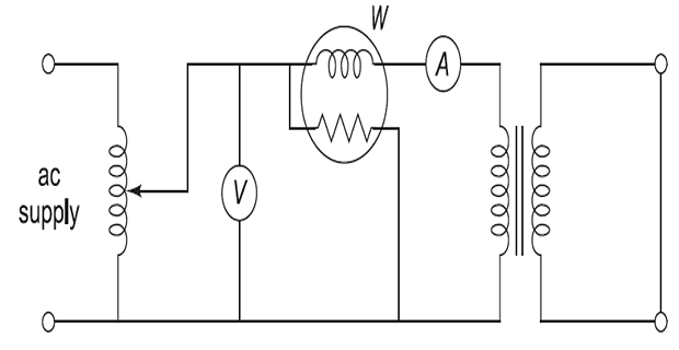
Short-Cicuit Test (SC)
-
Purpose : To determine
-
full-load copper loss
-
equivalent resistance ( \(R_{01}\) or \(R_{02}\) )
-
equivalent reactance ( \(X_{01}\) or \(X_{02}\) )
-
-
Test Connections :
-
LV side short-circuited while low-voltage is applied to other winding
-
Applied voltage slowly increased until F.L. current flows in the winding
-
Normally, the applied voltage is 5 to 10% of the rated voltage
-
Flux produced in core small & iron losses are very small.
-
Thus, wattmeter indicates full-load copper loss.
-