Transformer Efficiency: Losses & Equivalent Circuits

Losses in a Transformer

Types of losses in a transformer:
- Iron or core loss
- Copper loss
Iron loss:
- Due to the reversal of flux in the core
- Practically constant at all loads (no load to full load)
- Subdivided into two losses:
  - Hysteresis loss
  - Eddy-current loss
Hysteresis loss:
- Occurs due to the alternating flux in the core
- Depends on factors such as hysteresis loop area, core volume, and frequency of flux reversal

Eddy-current loss:
- Occurs due to the flow of eddy currents in the core
- Depends on factors such as lamination thickness, frequency of flux reversal, maximum flux density, core volume, and quality of magnetic material
- Eddy-current losses can be reduced by decreasing lamination thickness and adding silicon to steel.
Copper loss:
- due to the resistances of primary and secondary windings $\boxed{W_{C u}=I_{1}^{2}R_{1}+I_{2}^{2}R_{2}}$
- depends upon the load on the transformer
- proportional to square of load current of kVA rating

Ideal and Practical Transformers

For an ideal transformer:
1. No core loss and copper loss.
2. Winding resistance and leakage flux are zero.
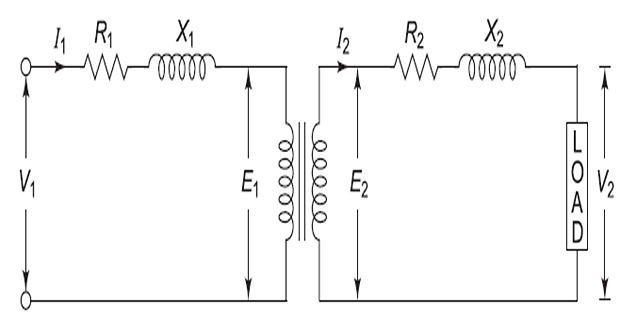
In a practical transformer:
1. The windings have some resistance.
2. There is always some leakage flux.

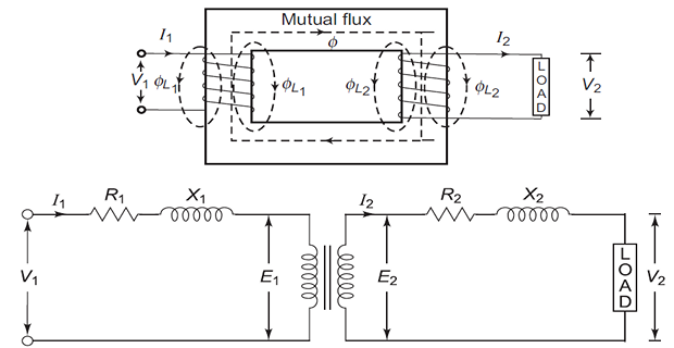
In an ideal transformer, it is assumed that all the flux produced by the primary winding links both the primary and secondary windings. However, in practice, this condition cannot be realized.
The flux $\phi_{L1}$ represents the primary leakage flux, which links only to the primary winding and does not link to the secondary winding.
Similarly, $\phi_{L2}$ is secondary leakage flux, which links only to the secondary winding and does not link to the primary winding.
The mutual flux, $\phi$ , links both the primary and secondary windings.

$\phi_{L1}$ is in phase with $I_1$ and produces a self-induced emf $E_{L1}$ in the primary winding.
$\phi_{L2}$ is in phase with $I_2$ and produces $E_{L2}$ in the secondary winding.
The induced voltages $E_{L1}$ and $E_{L2}$ caused by $\phi_{L1}$ and $\phi_{L2}$ differ from the induced voltages $E_1$ and $E_2$ caused by the main or mutual flux $\phi$ .
Leakage fluxes generate self-induced emfs in their respective windings.
Consequently, the leakage fluxes are equivalent to inductive coils connected in series with their respective windings.
The voltage drop in each series coil is equal to the voltage produced by the leakage flux. $E_{L_1}=I_1X_1~~\text{and}~~E_{L_2}=I_2X_2$

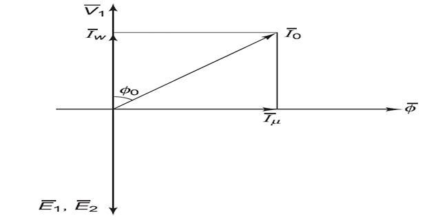
Phasor Diagram at No Load

No Load $\Rightarrow$ core loss and Cu loss in primary winding
$I_0$ supply core loss and very small Cu loss in primary
$I_0$ has two components:
- $I_\mu~\Rightarrow$ magnetising or reactive component
- $I_w~\Rightarrow$ power or active component
$I_\mu$ sets flux ( $\phi$ ) in the core and is in phase with $\phi$
$I_w$ responsible for power loss and phase with $V_1$

$\begin{aligned} I_\mu & = I_0\sin\phi_0 \\ I_w & = I_0\cos\phi_0\\ \bar{I}_0 & = \bar{I}_\mu + \bar{I}_w\\ I_0 & = \sqrt{I^2_\mu+I^2_w} \end{aligned}$

$I_0$ is very small as compared to $I_1$
copper loss negligible and $\boxed{W_0=W_i = V_1I_0\cos\phi_0}$

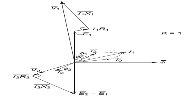
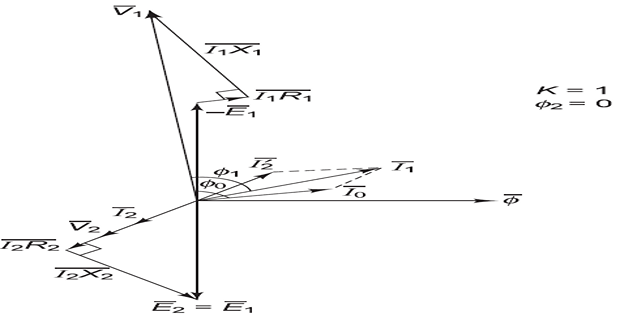
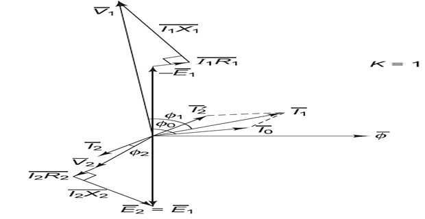
Phasor Diagram on Load

Load $\Rightarrow~I_2~\Rightarrow~\phi_2~\Rightarrow~\phi \downarrow~\Rightarrow~I_1 \uparrow ~\Rightarrow~\phi \uparrow ~\Rightarrow$ constant $\phi$
$I^{\prime}_2$ ( additional $I_1$ is anti-phase with $I_2$ ) sets $\phi^{\prime}_2$ cancel $\phi_2$ due to $I_2$

$\begin{gathered} {\frac{N_{2}}{N_{1}}}={\frac{I_{1}}{I_{2}}}={\frac{I_{0}+I_{2}^{\prime}}{I_{2}}}={\frac{I_{2}^{\prime}}{I_{2}}}=K \\ \boxed{I_1 = I_0+I^{\prime}_2 }\\ \boxed{I_2'=KI_2 } \end{gathered}$

$\begin{aligned} &\overline{{V_{1}}} =\overline{I_1R_1}+\overline{I_1X_1}+(-\overline{E_1}) \\ &\overline{E_2} =\overline{I_2R_2}+\overline{I_2X_2}+\overline{V_2} \\ &\overline{{I_1}} =\overline{I_0}+\overline{I_2'} \end{aligned}$

Transformer Efficiency: Losses & Equivalent Circuits

Demonstrative Video

Losses in a Transformer

Ideal and Practical Transformers

Phasor Diagram at No Load

Phasor Diagram on Load