Overview
Magnetic Circuits: Definition, Facts, and Applications
Introduction to Magnetic Circuits
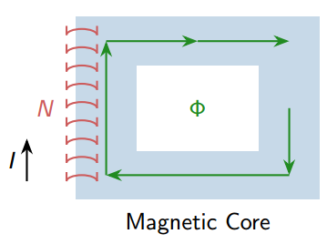
What is a Magnetic Circuit?
Definition: A closed path through which magnetic flux flows.
Key Components:
-
Magnetic core (iron, steel, ferrite)
-
Coil/winding carrying current
-
Air gaps (if any)
Applications:
-
Transformers
-
Electric motors & generators
-
Relays & solenoids
-
Inductors
Fundamental Quantities
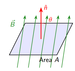
Magnetic Flux ( \(\Phi\) )
Definition: Total number of magnetic field lines passing through a surface.
Mathematical Expression \[\Phi = B \cdot A \cdot \cos\theta\]
Where:
-
\(\Phi\) = Magnetic flux (Wb)
-
\(B\) = Flux density (T or Wb/m 2 )
-
\(A\) = Cross-sectional area (m 2 )
-
\(\theta\) = Angle between \(\vec{B}\) and normal
Unit: Weber (Wb)
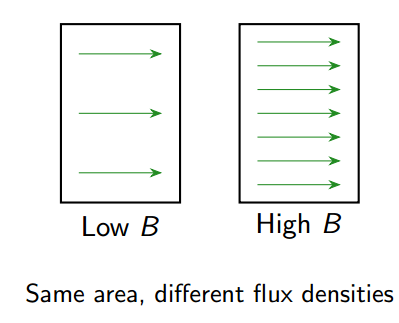
Magnetic Flux Density ( \(B\) )
Definition: Magnetic flux per unit area perpendicular to the field.
Formula \[B = \frac{\Phi}{A}\]
Physical Meaning:
-
Measures “concentration” of flux
-
Higher \(B\) \(\Rightarrow\) stronger field in region
-
Also called magnetic induction
Units:
-
SI: Tesla (T) = Wb/m 2
-
CGS: Gauss (G), where \(1\,\text{T} = 10^4\,\text{G}\)
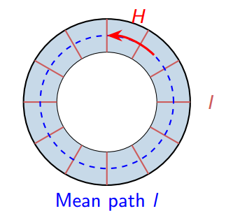
Magnetic Field Intensity ( \(H\) )
Definition: Measure of magnetizing force that creates the magnetic field.
From Ampère’s Law \[\oint \vec{H} \cdot d\vec{l} = NI\] For uniform field in mean path \(l\) : \[H = \frac{NI}{l}\]
Where:
-
\(H\) = Field intensity (A/m or At/m)
-
\(N\) = Number of turns
-
\(I\) = Current (A)
-
\(l\) = Mean path length (m)
MMF, Reluctance, and Permeability
Magnetomotive Force (MMF)
Definition: The “driving force” that establishes magnetic flux in a circuit.
MMF Formula \[\mathcal{F} = NI\]
Analogy with Electric Circuits:
| Electric | Magnetic |
|---|---|
| EMF \((V)\) | MMF \((\mathcal{F})\) |
Unit: Ampere-turns (At)
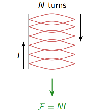
Note Think of MMF as the “magnetic pressure” pushing flux through the circuit.
Reluctance ( \(\mathcal{R}\) )
Definition: Opposition offered by a magnetic circuit to the flow of flux.
Reluctance Formula \[\mathcal{R} = \frac{l}{\mu_0 \mu_r A} = \frac{l}{\mu A}\]
Where:
-
\(l\) = Length of magnetic path (m)
-
\(A\) = Cross-sectional area (m 2 )
-
\(\mu_0 = 4\pi \times 10^{-7}\) H/m
-
\(\mu_r\) = Relative permeability
Unit: At/Wb or H −1
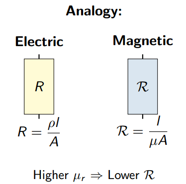
Analogy:
Higher \(\mu_r\) \(\Rightarrow\) Lower \(\mathcal{R}\)
Permeability ( \(\mu\) )
Definition: Measure of a material’s ability to support magnetic flux.
Relationship \[B = \mu H = \mu_0 \mu_r H\]
Types:
-
\(\mu_0\) = Permeability of free space
\(= 4\pi \times 10^{-7}\) H/m -
\(\mu_r\) = Relative permeability (dimensionless)
-
\(\mu = \mu_0 \mu_r\) = Absolute permeability
| Material | \(\mu_r\) |
|---|---|
| Air/Vacuum | 1 |
| Soft Iron | 2000–8000 |
| Silicon Steel | 5000–10000 |
| Cast Iron | 100–300 |
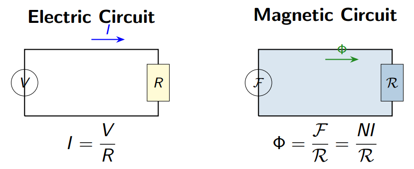
Ohm’s Law for Magnetic Circuits
Ohm’s Law for Magnetic Circuits (Rowland’s Law)
| Electric | Magnetic | Relation |
|---|---|---|
| EMF ( \(V\) ) | MMF ( \(\mathcal{F} = NI\) ) | Driving force |
| Current ( \(I\) ) | Flux ( \(\Phi\) ) | Flow quantity |
| Resistance ( \(R\) ) | Reluctance ( \(\mathcal{R}\) ) | Opposition |
Complete Electric-Magnetic Analogy
| Quantity | Electric | Magnetic | Unit (Mag) |
|---|---|---|---|
| Driving Force | EMF ( \(V\) ) | MMF ( \(\mathcal{F}=NI\) ) | At |
| Response | Current ( \(I\) ) | Flux ( \(\Phi\) ) | Wb |
| Opposition | Resistance ( \(R\) ) | Reluctance ( \(\mathcal{R}\) ) | At/Wb |
| Intensity | Current density ( \(J\) ) | Flux density ( \(B\) ) | T |
| Field | Electric field ( \(E\) ) | Field intensity ( \(H\) ) | At/m |
| Material property | Conductivity ( \(\sigma\) ) | Permeability ( \(\mu\) ) | H/m |
| Ohm’s Law | \(V = IR\) | \(\mathcal{F} = \Phi\mathcal{R}\) | – |
Important Note Unlike electric current, magnetic flux does not actually “flow” — it is a static field pattern. The analogy is for calculation convenience only!
Series and Parallel Magnetic Circuits
Series Magnetic Circuit
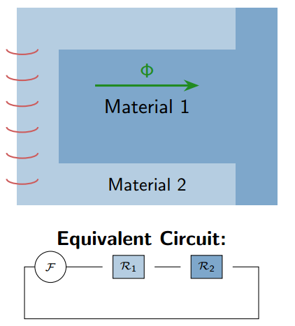
Key Points:
-
Same flux \(\Phi\) through all sections
-
MMF drops add up
Series Reluctance \[\mathcal{R}_{eq} = \mathcal{R}_1 + \mathcal{R}_2 + \mathcal{R}_3 + \cdots\]
MMF Equation \[\mathcal{F} = \Phi(\mathcal{R}_1 + \mathcal{R}_2 + \cdots)\] \[NI = H_1 l_1 + H_2 l_2 + \cdots\]
Parallel Magnetic Circuit
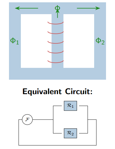
Key Points:
-
Flux divides: \(\Phi = \Phi_1 + \Phi_2\)
-
Same MMF across parallel paths
Parallel Reluctance \[\frac{1}{\mathcal{R}_{eq}} = \frac{1}{\mathcal{R}_1} + \frac{1}{\mathcal{R}_2}\]
For Two Parallel Paths \[\mathcal{R}_{eq} = \frac{\mathcal{R}_1 \cdot \mathcal{R}_2}{\mathcal{R}_1 + \mathcal{R}_2}\]
Air Gaps in Magnetic Circuits
Effect of Air Gap
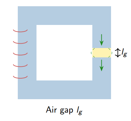
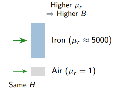
Why Air Gap Matters:
-
\(\mu_r\) of air \(= 1\) (vs. iron \(\approx\) 5000)
-
Air gap has very high reluctance
-
Small gap \(\Rightarrow\) large MMF drop
Air Gap Reluctance \[\mathcal{R}_g = \frac{l_g}{\mu_0 A_g}\]
Fringing Effect:
-
Flux spreads out at air gap
-
Effective area increases
-
Often neglected for small gaps
Fringing Effect – Quantitative Analysis
Fringing Factor ( \(k_f\) ):
-
Flux spreads beyond core area
-
Effective gap area \(>\) core area
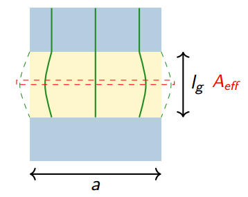
Rule of Thumb For small gaps, add \(l_g\) to each linear dimension of the gap area.
Empirical Correction For rectangular core ( \(a \times b\) ): \[A_{eff} = (a + l_g)(b + l_g)\]
Fringing factor: \[k_f = \frac{A_{eff}}{A_{core}} = \frac{(a+l_g)(b+l_g)}{ab}\]
Corrected Gap Reluctance: \[\mathcal{R}_g = \frac{l_g}{\mu_0 A_{eff}} = \frac{l_g}{\mu_0 k_f A}\]
Magnetic Circuit with Air Gap – Analysis
Total Reluctance: \[\mathcal{R}_{total} = \mathcal{R}_{core} + \mathcal{R}_{gap}\] \[\mathcal{R}_{total} = \frac{l_c}{\mu_0 \mu_r A_c} + \frac{l_g}{\mu_0 A_g}\]
Total MMF Required: \[NI = \Phi \cdot \mathcal{R}_{total}\] \[NI = H_c l_c + H_g l_g\]
Since \(B_g = \mu_0 H_g\) : \[H_g = \frac{B_g}{\mu_0} = \frac{B}{\mu_0}\]
(Assuming no fringing: \(B_g = B_c = B\) )
Typical Values For a circuit with:
-
\(l_c = 0.5\) m (core)
-
\(l_g = 1\) mm (gap)
-
\(\mu_r = 5000\)
Ratio of reluctances: \[\frac{\mathcal{R}_g}{\mathcal{R}_c} = \frac{l_g \cdot \mu_r}{l_c}\] \[= \frac{0.001 \times 5000}{0.5} = 10\]
A 1 mm gap has 10 \(\times\) the reluctance of 0.5 m of iron!
Leakage Flux
Leakage Flux and Leakage Factor
Definitions:
-
Useful flux ( \(\Phi_u\) ): Flux linking both coils or passing through intended path
-
Leakage flux ( \(\Phi_l\) ): Flux that takes path through air
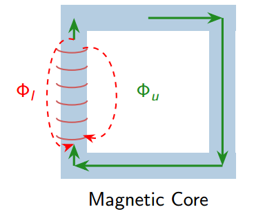
Total Flux \[\Phi_{total} = \Phi_u + \Phi_l\]
Leakage Factor ( \(\lambda\) ) \[\lambda = \frac{\Phi_{total}}{\Phi_u} = \frac{\Phi_u + \Phi_l}{\Phi_u}\] \[\lambda = 1 + \frac{\Phi_l}{\Phi_u} > 1\]
Typical values: \(\lambda = 1.1\) to \(1.25\)
Leakage Flux – Practical Implications
Why Leakage Matters:
-
Reduces useful flux available
-
Lowers transformer/machine efficiency
-
Causes voltage drops in transformers
-
Affects coupling between windings
Design Consideration MMF required at source: \[\mathcal{F} = \Phi_u \cdot \mathcal{R}_{core} \cdot \lambda\]
Or accounting for leakage: \[NI = \lambda \cdot \Phi_u \cdot \mathcal{R}\]
Minimizing Leakage:
-
Use high-permeability core
-
Minimize air gaps
-
Place windings close together
-
Use interleaved windings
-
Proper core geometry design
Leakage Coefficient \[\sigma = 1 - \frac{1}{\lambda} = \frac{\Phi_l}{\Phi_{total}}\] Represents fraction of flux that leaks.
B-H Curve and Hysteresis
B-H Curve (Magnetization Curve)
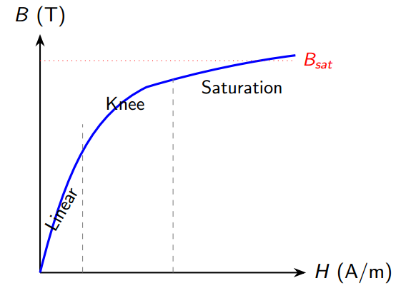
Machines designed to operate at knee for efficiency.
Three Regions:
1. Linear Region:
-
\(B \propto H\) (constant \(\mu\) )
-
Domains align gradually
2. Knee Region:
-
Transition zone
-
\(\mu\) starts decreasing
3. Saturation Region:
-
All domains aligned
-
\(B\) increases very slowly
-
\(\mu \rightarrow \mu_0\)
Hysteresis Loop
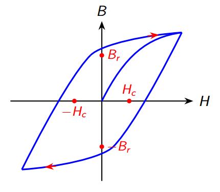
Key Parameters:
Retentivity ( \(B_r\) ):
-
Residual flux when \(H = 0\)
-
Material “remembers” magnetization
Coercivity ( \(H_c\) ):
-
\(H\) needed to demagnetize
-
Reverse field to make \(B = 0\)
Loop Area = Energy Loss
-
Dissipated as heat per cycle
-
Hysteresis loss \(\propto\) frequency
Hysteresis Loss
Energy lost per cycle = Area of hysteresis loop
Steinmetz Equation \[P_h = \eta \cdot B_{max}^n \cdot f \cdot V\]
Where:
-
\(P_h\) = Hysteresis loss (W)
-
\(\eta\) = Steinmetz coefficient
-
\(B_{max}\) = Maximum flux density (T)
-
\(n\) = Steinmetz exponent ( \(\approx 1.6\) – \(2.0\) )
-
\(f\) = Frequency (Hz)
-
\(V\) = Volume of core (m 3 )
Eddy Currents
Eddy Currents
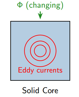
What are Eddy Currents?
-
Circulating currents induced in conductor
-
Caused by changing magnetic flux
-
Follow Lenz’s Law (oppose change)
Effects:
-
Power loss ( \(I^2R\) heating)
-
Useful in induction heating
-
Useful in electromagnetic braking
Eddy Current Loss \[P_e = K_e \cdot B_{max}^2 \cdot f^2 \cdot t^2 \cdot V\] where \(t\) = thickness of lamination
Reducing Eddy Current Losses – Laminations
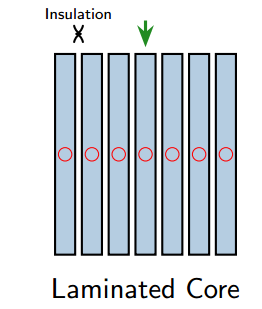
Laminations oriented parallel to flux direction.
Why Laminations Work:
-
Core divided into thin sheets
-
Each sheet insulated (varnish/oxide)
-
Eddy current paths broken
-
Smaller loops \(\Rightarrow\) higher resistance
Key Points:
-
\(P_e \propto t^2\) (thickness squared)
-
Thinner laminations = less loss
-
Typical: 0.35–0.5 mm thick
-
Used in transformers, motors
Core Losses – Combined Analysis
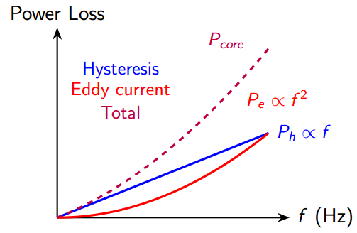
Separation Method: \[\frac{P_{core}}{f} = k_h B_{max}^n + k_e B_{max}^2 f \cdot t^2\] Plot \(\frac{P_{core}}{f}\) vs \(f\) \(\Rightarrow\) straight line
Total Core Loss \[P_{core} = P_h + P_e\] \[P_{core} = k_h B_{max}^n f + k_e B_{max}^2 f^2 t^2\]
Key Observations:
-
At low frequency : \(P_h\) dominates
-
At high frequency : \(P_e\) dominates
-
Crossover depends on lamination thickness
Core Loss – Design Guidelines
To Reduce Hysteresis Loss:
-
Use soft magnetic materials
-
Choose materials with narrow B-H loop
-
Silicon steel (3–4% Si) preferred
-
Grain-oriented steel for transformers
To Reduce Eddy Current Loss:
-
Use laminated cores
-
Thinner laminations for higher frequency
-
Add silicon to increase resistivity
-
Use ferrites at very high frequencies
Typical Lamination Thickness
| Application | Thickness |
|---|---|
| Power transformers | 0.35–0.5 mm |
| (50/60 Hz) | |
| Small motors | 0.35–0.65 mm |
| High-speed motors | 0.2–0.35 mm |
| Aircraft (400 Hz) | 0.1–0.2 mm |
| High frequency | Ferrite cores |
| ( \(>\) 10 kHz) | (no laminations) |
Thinner = less eddy loss but higher cost
Magnetic Materials
Classification of Magnetic Materials
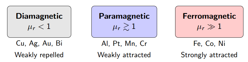
For Electrical Machines: Ferromagnetic materials are essential!
-
High permeability concentrates flux
-
Enables strong magnetic fields with less current
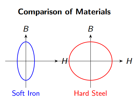
Soft vs Hard Magnetic Materials
Soft Magnetic Materials Properties:
-
Easy to magnetize/demagnetize
-
Low coercivity ( \(H_c\) )
-
Narrow hysteresis loop
-
Low hysteresis loss
Examples:
Silicon steel, soft iron, permalloy
Applications:
Transformer cores, motor cores, electromagnets
Hard Magnetic Materials Properties:
-
Difficult to demagnetize
-
High coercivity ( \(H_c\) )
-
Wide hysteresis loop
-
High retentivity ( \(B_r\) )
Examples:
Alnico, ferrites, NdFeB, SmCo
Applications:
Permanent magnets, speakers, hard drives
Solved Example
A magnetic circuit has a mean length of 50 cm and cross-sectional area of 4 cm 2 . It includes an air gap of 1 mm. The core has \(\mu_r = 2000\) . Find the current required in a 500-turn coil to produce a flux of 0.4 mWb.
Given:
\(l_c = 0.5 - 0.001 = 0.499\)
m,
\(l_g = 0.001\)
m,
\(A = 4 \times 10^{-4}\)
m
2
\(\mu_r = 2000\)
,
\(N = 500\)
,
\(\Phi = 0.4 \times 10^{-3}\)
Wb
Solution: \[\begin{aligned} \mathcal{R}_{core} &= \frac{l_c}{\mu_0 \mu_r A} = \frac{0.499}{4\pi \times 10^{-7} \times 2000 \times 4 \times 10^{-4}} = 4.97 \times 10^5 \text{ At/Wb}\\[0.2cm] \mathcal{R}_{gap} &= \frac{l_g}{\mu_0 A} = \frac{0.001}{4\pi \times 10^{-7} \times 4 \times 10^{-4}} = 1.99 \times 10^6 \text{ At/Wb}\\[0.2cm] \mathcal{R}_{total} &= 4.97 \times 10^5 + 1.99 \times 10^6 = 2.49 \times 10^6 \text{ At/Wb}\\[0.2cm] NI &= \Phi \times \mathcal{R}_{total} = 0.4 \times 10^{-3} \times 2.49 \times 10^6 = 996 \text{ At}\\[0.2cm] I &= \frac{996}{500} = \boxed{1.99 \text{ A}} \end{aligned}\]
Practice Problem
A ring-shaped iron core has a mean circumference of 80 cm and a cross-sectional area of 5 cm 2 . It has two air gaps, each 1.5 mm wide. A coil of 600 turns is wound on the core. The relative permeability of iron is 1500. Neglecting leakage and fringing, calculate:
-
The total reluctance of the magnetic circuit
-
The current required to produce a flux of 0.5 mWb
-
The flux density in the core and air gap
Hints:
-
Core length \(l_c = 0.8 - 2(0.0015) = 0.797\) m
-
Two air gaps in series: \(\mathcal{R}_{gap,total} = 2\mathcal{R}_{gap}\)
-
Use \(\Phi = \mathcal{F}/\mathcal{R}_{total}\) to find current
Answers: (a) \(5.84 \times 10^6\) At/Wb (b) 4.87 A (c) 1 T
Summary
Key Formulas Summary
| Quantity | Formula | Unit |
|---|---|---|
| Magnetic Flux | \(\Phi = BA\) | Wb |
| Flux Density | \(B = \mu H = \mu_0 \mu_r H\) | T |
| Field Intensity | \(H = \dfrac{NI}{l}\) | A/m |
| MMF | \(\mathcal{F} = NI\) | At |
| Reluctance | \(\mathcal{R} = \dfrac{l}{\mu_0 \mu_r A}\) | At/Wb |
| Ohm’s Law (Mag) | \(\Phi = \dfrac{\mathcal{F}}{\mathcal{R}} = \dfrac{NI}{\mathcal{R}}\) | – |
| Series Reluctance | \(\mathcal{R}_{eq} = \mathcal{R}_1 + \mathcal{R}_2 + \cdots\) | At/Wb |
| Parallel Reluctance | \(\dfrac{1}{\mathcal{R}_{eq}} = \dfrac{1}{\mathcal{R}_1} + \dfrac{1}{\mathcal{R}_2}\) | At/Wb |
Key Takeaways
-
Magnetic circuits are analogous to electric circuits — MMF drives flux through reluctance.
-
Permeability determines how easily a material supports magnetic flux.
-
Air gaps dramatically increase reluctance — even small gaps dominate the circuit.
-
B-H curve shows nonlinear behavior; saturation limits maximum flux density.
-
Hysteresis loss occurs due to domain realignment; minimized using soft magnetic materials.
-
Eddy current loss reduced by using laminated cores.
-
Core losses = Hysteresis loss + Eddy current loss (important for efficiency).