Set 20 — Efficiency and All-Day Efficiency
A transformer loses power in two places and nowhere else. The core loses it to hysteresis and eddy currents at a rate fixed by the flux, which the supply holds constant; the windings lose it to their own resistance at a rate that follows the square of the current. Every efficiency question in this set is an exercise in keeping those two apart and then adding them back at the right load.
The consequences are worth more than the arithmetic. Because one loss is fixed and the other grows, the efficiency has a maximum, and it falls at the load where the two are equal — a load the designer chooses when specifying the core. The last problem takes that idea to its practical conclusion: a distribution transformer is energised for 24 hours whatever its customers do, so it is judged on kilowatt-hours rather than kilowatts.
Efficiency is output over input, and the input is always the output plus the two losses:
\[ \eta = \frac{P_{\text{out}}}{P_{\text{out}} + P_i + P_{cu}} = \frac{xS\cos\phi}{xS\cos\phi + P_i + x^2P_{cu,\text{FL}}} \]\(x\) is the fraction of full load, \(S\) the rating in kVA and \(\cos\phi\) the load power factor.
One loss is constant, the other is not. Iron loss is fixed by the flux, which is fixed by \(V/f\); copper loss follows the square of the current:
\[ P_i = \text{constant}, \qquad P_{cu} = x^2P_{cu,\text{FL}} \]Maximum efficiency occurs where the two losses are equal. Setting \(d\eta/dx = 0\) gives \(P_i = x^2P_{cu,\text{FL}}\), so
\[ x_{\max} = \sqrt{\frac{P_i}{P_{cu,\text{FL}}}}, \qquad \text{kVA at }\eta_{\max} = S\sqrt{\frac{P_i}{P_{cu,\text{FL}}}} \]The power factor moves the value of the efficiency but not its location. \(\cos\phi\) multiplies the output only; the losses depend on current, so \(x_{\max}\) is a property of the machine alone.
Copper loss is set by the kVA, never by the kW. A load quoted in kilowatts must be divided by its own power factor before the \(x^2\) rule is applied.
All-day efficiency is a ratio of energies over 24 hours, not of powers at an instant:
\[ \eta_{\text{all-day}} = \frac{\text{output kWh in 24 h}}{\text{output kWh} + \text{copper kWh} + 24P_i} \]The iron loss term runs for the full 24 hours because the primary stays energised even when nothing is drawn.
An 11000/230 V, 150 kVA, single-phase, 50 Hz transformer has a core loss of 1.4 kW and a full-load copper loss of 1.6 kW. Determine
- the kVA load for maximum efficiency and the value of that maximum efficiency at unity power factor
- the efficiency at half full load and 0.8 power factor leading.
Maximum efficiency happens where the variable loss has grown to equal the fixed loss. With \(x\) the fraction of full load:
Note which loss is on top. The iron loss is the numerator, because it is the constant that the copper loss has to catch up with.
The corresponding load is that fraction of the rating:
At that load the two losses are equal, so the total is simply twice the iron loss:
Now part (ii), at half load. The copper loss falls with the square of the current while the iron loss does not move at all:
The output at half load and 0.8 power factor:
That the power factor is leading changes nothing in this calculation. Losses depend on the magnitude of the current, and 0.8 leading draws exactly the current that 0.8 lagging does.
Why the second answer is the lower one, even though 0.94 and 0.5 of full load are both away from nothing: the loss has fallen from 2.8 kW to 1.8 kW, but the output has fallen from 140.3 kW to 60 kW — much faster. Efficiency is a ratio, and the loss per unit of output is what actually rises.
A 20 kVA, 440/220 V, single-phase, 50 Hz transformer has an iron loss of 324 W. The copper loss is found to be 100 W when the transformer delivers half full-load current. Determine
- the efficiency when delivering full-load current at 0.8 power factor lagging
- the percentage of full load at which the efficiency is a maximum.
Scale the copper loss up to full load first. It is quoted at half current, and copper loss goes as the square of current:
Doubling the current quadruples the loss. Doubling 100 W to 200 W is the most common error in this set.
Total loss at full load, the iron loss being unchanged by the load:
Full-load output at 0.8 power factor, and the efficiency:
The load for maximum efficiency comes straight from the loss ratio:
How much is actually gained by moving to that load, at the same 0.8 power factor:
Two hundredths of a percent above the full-load figure. The efficiency curve is extremely flat near its peak, which is why the exact location of \(x_{\max}\) matters far less in practice than it does in examinations.
A 600 kVA single-phase transformer has an efficiency of 92% at both full load and half load at unity power factor. Determine its efficiency at 60% of full load and 0.8 power factor lagging.
Write the efficiency in its general form, because the two given conditions are two instances of the same equation with different \(x\):
Two unknowns, \(P_i\) and \(P_{cu}\); two given efficiencies. The problem is a pair of simultaneous equations in disguise.
At full load, unity power factor — here \(x = 1\):
At half load, unity power factor — here \(x = \tfrac12\), so the copper loss is quartered:
Subtract (ii) from (i) to separate the two losses:
The full-load copper loss is exactly twice the iron loss — which is what "equal efficiency at \(x\) and \(x/2\)" always forces, whatever the numbers.
Now evaluate at \(x = 0.6\) and 0.8 power factor:
Locate the peak, as a check on the loss split. Maximum efficiency sits at
The peak lies at the geometric mean of the two loads given, \(\sqrt{1\times0.5} = 0.707\) — as it must, since the efficiency curve is symmetric in \(\ln x\) about its maximum. Two loads with equal efficiency are always placed symmetrically about \(x_{\max}\).
Find the all-day efficiency of a 500 kVA distribution transformer whose copper loss and iron loss at full load are 4.5 kW and 3.5 kW respectively. During a day of 24 hours it is loaded as under:
| Duration | Load | Power factor |
|---|---|---|
| 6 hours | 400 kW | 0.8 |
| 10 hours | 300 kW | 0.75 |
| 4 hours | 100 kW | 0.8 |
| 4 hours | No load | — |
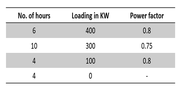
Convert every load to kVA before anything else. Copper loss follows the current, and the current follows the kVA — the kilowatts alone say nothing until the power factor is divided out:
The 300 kW block is the trap: it is a smaller load in kilowatts than the first but at a poorer power factor, so it still draws 80% of rated current.
Copper loss at each of those loads, scaled from the full-load value by the square of the kVA ratio:
Total copper loss over the day, each figure multiplied by the hours it lasts:
Iron loss over the day. It is present for all 24 hours, including the four with no load at all, because the primary stays connected to the supply:
The iron loss is 60% of the day's total loss even though it is the smaller of the two full-load figures. That single fact is the reason for the whole concept of all-day efficiency.
Energy delivered over the day, in kilowatt-hours — the kW figures are used here, not the kVA:
The all-day efficiency:
Compare with the ordinary efficiency at the peak of the cycle, 400 kW at 0.8:
Higher than the all-day figure, and it would be quoted on the nameplate. The 0.4 percentage points between them is the price of fourteen hours spent at part load or none.
Key Formulas
| Quantity | Relation | Notes |
|---|---|---|
| Efficiency | \(\eta = \dfrac{P_{\text{out}}}{P_{\text{out}} + P_i + P_{cu}}\) | Every problem on the page |
| Output at part load | \(P_{\text{out}} = xS\cos\phi\) | \(x\) = fraction of full load — Problems 1, 3 |
| Copper loss scaling | \(P_{cu} = x^2P_{cu,\text{FL}}\) | Square law, not linear — Problems 1, 2, 3, 4 |
| Copper loss from a test | \(P_{cu,\text{FL}} = P_{cu}(x)/x^2\) | 400 W from 100 W at half load — Problem 2 |
| Iron loss | \(P_i = \text{constant}\) | Fixed by \(V/f\), independent of load |
| Condition for \(\eta_{\max}\) | \(x^2P_{cu,\text{FL}} = P_i\) | Variable loss equals constant loss |
| Load at \(\eta_{\max}\) | \(x_{\max} = \sqrt{P_i/P_{cu,\text{FL}}}\) | 0.935 in Problem 1, 0.9 in Problem 2, 0.707 in Problem 3 |
| kVA at \(\eta_{\max}\) | \(S\sqrt{P_i/P_{cu,\text{FL}}}\) | 140.3 kVA in Problem 1 |
| Maximum efficiency | \(\eta_{\max} = \dfrac{x_{\max}S\cos\phi}{x_{\max}S\cos\phi + 2P_i}\) | Total loss is twice the iron loss there — Problems 1, 3 |
| Equal efficiency at two loads | \(x_1x_2 = P_i/P_{cu,\text{FL}}\) | Splits the losses in one line — Problem 3 |
| kVA from a kW load | \(S = \text{kW}/\cos\phi\) | Required before any \(x^2\) scaling — Problem 4 |
| Copper energy in a day | \(W_{cu} = \sum t_kP_{cu,k}\) | Block by block — Problem 4 |
| Iron energy in a day | \(W_i = 24P_i\) | All 24 hours, no-load periods included — Problem 4 |
| All-day efficiency | \(\eta_{\text{all-day}} = \dfrac{\sum t_kP_{\text{out},k}}{\sum t_kP_{\text{out},k} + W_{cu} + W_i}\) | Energies, not powers — Problem 4 |
Common Mistakes
Inverting the ratio under the root. The load for maximum efficiency is \(\sqrt{P_i/P_{cu}}\), not \(\sqrt{P_{cu}/P_i}\); in Problem 1 the two give 140.3 kVA and 160.4 kVA, and only the first can be right because the iron loss is the smaller of the two.
Scaling the copper loss linearly. Half current gives a quarter of the loss, so the 100 W of Problem 2 becomes 400 W at full load, not 200 W.
Scaling the copper loss on kilowatts instead of kilovolt-amperes. In Problem 4 the 300 kW block at 0.75 power factor is 400 kVA, and using \((300/400)^2\) instead of \((400/500)^2\) understates its copper loss by 37%.
Letting the iron loss stop when the load does. The four idle hours of Problem 4 still cost 14 kWh of core loss, because the primary remains energised.
Putting the power factor into a loss term. \(\cos\phi\) multiplies the output only; the 0.8 leading of Problem 1 gives exactly the same losses as 0.8 lagging.
Assuming maximum efficiency occurs at full load. It occurs where the losses are equal, which is 90% of full load in Problem 2 and 70.7% in Problem 3.
Reading "equal efficiency at two loads" as "maximum efficiency at those loads". In Problem 3 both are 92% while the true peak between them is 92.42%.
Mixing watts and kilowatts in the same fraction. Problem 2 has an output of 16 kW and a loss of 724 W; one of them has to be converted before they are added.
Computing an all-day efficiency from powers. It is a ratio of kilowatt-hours; averaging the four instantaneous efficiencies of Problem 4 gives a different and meaningless number.
Quoting the all-day efficiency as the transformer's efficiency. The nameplate figure for Problem 4 is 98.04% at its peak load; the all-day value of 97.63% describes the duty cycle as much as the machine.
Two numbers — a constant iron loss and a full-load copper loss — have now been made to answer every question about how a transformer performs. Set 19 used the series resistance and reactance for the voltage drop; this set used the same resistance for the loss, added the shunt branch's iron loss, and turned the pair into an efficiency curve with a peak whose position the designer chooses.
One machine has been considered in isolation throughout. Substations do not work that way: transformers are banked in parallel so that units can be taken out for maintenance and so that the plant can grow with the load. The moment two of them share a busbar, their impedances decide how the load divides, their ratios decide whether a circulating current flows with no load connected at all, and their percentage values — the ones computed in Set 19 — become the whole story.
Next: Set 21 — Parallel Operation and Load Sharing, where the conditions for paralleling are set out and the load is divided between unequal transformers.