Set 36 — Voltage Regulation — EMF, MMF and ZPF Methods
Load an alternator and its terminal voltage changes, because the armature current drops voltage across the winding resistance and the synchronous reactance. Regulation is the size of that change, measured with the excitation and the speed held fixed, and computing it means adding two phasors to the terminal voltage — nothing more.
What varies from problem to problem is the sign and the source of \(X_s\). A lagging load makes the reactance drop add to the terminal voltage and the regulation positive; a leading load makes it subtract, and the regulation can go negative. The reactance itself may be given, or measured by the synchronous-impedance method from open- and short-circuit tests, or extracted from a zero-power-factor test. This set works through all three routes and keeps every quantity per phase.
Regulation is defined at constant excitation and constant speed. Throw off the load and the terminal voltage rises from \(V\) to \(E_f\); the rise expressed as a fraction is the regulation:
\[ \%\,\text{regulation} = \frac{E_f - V}{V}\times 100 \]Both voltages are per phase. Mixing a line value with a phase value here is the fastest way to a wrong answer.
The per-phase equation is one phasor sum. With the terminal voltage taken as reference and the load current lagging by \(\phi\):
\[ \mathbf{E}_f = \mathbf{V} + \mathbf{I}_a(R_a + jX_s) \]Resolved along and across \(\mathbf{V}\) it becomes the working formula, the sign taking care of the power factor:
\[ E_f = \sqrt{\left(V\cos\phi + I_aR_a\right)^2 + \left(V\sin\phi \pm I_aX_s\right)^2} \]Plus for a lagging load, minus for a leading one. A sufficiently leading load makes \(E_f < V\) and the regulation negative.
Resolving along the current instead gives the same magnitude and the load angle directly — useful when \(\delta\) is wanted:
\[ E_\parallel = V + I_aR_a\cos\phi + I_aX_s\sin\phi, \qquad E_\perp = I_aX_s\cos\phi - I_aR_a\sin\phi \]\[ E_f = \sqrt{E_\parallel^2 + E_\perp^2}, \qquad \delta = \tan^{-1}\frac{E_\perp}{E_\parallel} \]The e.m.f. (synchronous impedance) method obtains \(X_s\) from an open-circuit and a short-circuit test taken at the same field current:
\[ Z_s = \frac{\text{O.C. voltage per phase}}{\text{S.C. current per phase}}, \qquad X_s = \sqrt{Z_s^2 - R_a^2} \]The open-circuit voltage is read on the unsaturated part of the curve, so \(X_s\) comes out too large and the method is pessimistic — it over-estimates the regulation.
The m.m.f. (ampere-turn) method adds field m.m.f.s instead of voltages, treats the machine as fully saturated, and is correspondingly optimistic. The true regulation lies between the two.
The zero-power-factor (Potier) test loads the machine at rated current with a purely reactive load. At \(\cos\phi = 0\) the reactance drop lies wholly along \(\mathbf{V}\), so the phasor triangle collapses into a scalar subtraction and the reactance can be read off directly.
Armature reaction hides inside \(X_s\). The synchronous reactance is the sum of the true leakage reactance and a fictitious reactance representing the armature's own field:
\[ X_s = X_L + X_a \]
A 3-phase, star-connected alternator supplies a load of 10 MW at 0.85 power factor lagging and at a terminal voltage of 11 kV. Its armature resistance is 0.1 Ω per phase and its synchronous reactance 0.66 Ω per phase. Calculate the line value of the generated e.m.f.
Line current from the three-phase power. The 10 MW is the power of all three phases together, so the \(\sqrt3\) belongs in the denominator:
Reduce everything to one phase. The impedances are quoted per phase, so the voltage must be too:
The power-factor angle:
Add the drops as phasors, taking \(\mathbf V\) as reference and the load lagging:
Return to a line value, which is what the question asked for:
The corresponding regulation is \((6625-6351)/6351 = 4.3\ \%\) — small, because the per-unit reactance of this machine is low.
In a 50 kVA, star-connected, 440 V, 3-phase, 50 Hz alternator the effective armature resistance is 0.25 Ω per phase, the synchronous reactance is 3.2 Ω per phase and the leakage reactance is 0.5 Ω per phase. At rated load and unity power factor determine
- the internal e.m.f. \(E_a\) behind the leakage reactance;
- the no-load e.m.f. \(E_f\);
- the percentage regulation on full load;
- the value of reactance which replaces armature reaction.
Per-phase quantities. At unity power factor the whole rated kVA is real power, and the current follows from the kVA rating:
The three voltage drops:
(a) Internal e.m.f. This is the voltage behind the resistance and the leakage reactance only — the e.m.f. actually induced by the resultant air-gap flux. At unity power factor \(\cos\phi = 1\), \(\sin\phi = 0\), so the resistive drop is in phase with \(\mathbf V\) and the reactive drop in quadrature:
(b) No-load e.m.f. The same construction with the synchronous reactance, which additionally accounts for armature reaction:
(c) Regulation. Per phase throughout:
Large, and it would be just as large computed on the line values — the \(\sqrt3\) cancels in a ratio. Note that even at unity power factor the regulation is heavy, because \(X_s\) is 0.83 p.u. on this machine's own base.
(d) The armature-reaction reactance is what is left of \(X_s\) after the genuine leakage is removed:
Armature reaction accounts for 84 % of the synchronous reactance here. It is not a stray effect but the dominant one, and that is why \(X_s\) rather than \(X_L\) governs the terminal behaviour.
A 1000 kVA, 3300 V, 3-phase, star-connected alternator delivers full-load current at rated voltage and 0.80 power factor lagging. The resistance and synchronous reactance per phase are 0.5 Ω and 5 Ω respectively. Estimate the generated voltage and the load angle.
Per-phase quantities from the rating:
Note the kVA, not the kW, gives the current directly — no power factor is involved in that step.
Resolve the two drops along \(\mathbf V\). The resistive drop is in phase with \(\mathbf I_a\), which lags \(\mathbf V\) by \(\phi\); the reactive drop leads \(\mathbf I_a\) by 90°. Their components along \(\mathbf V\) are therefore
And at right angles to \(\mathbf V\), where the two drops oppose one another:
The minus sign is not optional. With a lagging current the resistive drop has a component behind \(\mathbf V\), and adding it instead of subtracting gives 752.5 V and a load angle 3° too large.
The generated e.m.f. is the hypotenuse:
The load angle is the angle by which \(\mathbf E_f\) leads \(\mathbf V\):
Equivalently \(\delta = \sin^{-1}(647.5/2582.5) = 14.5^\circ\). This is the angle that carries the power: \(P \approx 3E_fV\sin\delta/X_s\), a relation Set 38 leans on heavily.
The regulation follows at once:
A 100 kVA, 3000 V, 50 Hz, 3-phase star-connected alternator has an effective armature resistance of 0.2 Ω per phase. A field current of 40 A produces a short-circuit current of 200 A and an open-circuit e.m.f. of 1040 V (line value). Calculate the full-load voltage regulation at 0.8 power factor lagging and at 0.8 power factor leading, and describe the phasor diagrams.
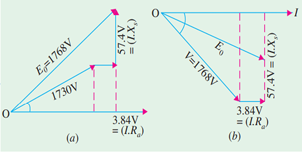
Synchronous impedance from the two tests. Both readings are taken at the same field current of 40 A, which is what makes the ratio meaningful. The open-circuit figure is a line value and must be reduced to a phase value first:
Separate the reactance:
With \(R_a \ll X_s\) the reactance is barely distinguishable from the impedance — typical of any machine above a few kVA, and a useful sanity check.
Full-load conditions per phase:
0.8 power factor lagging. The reactive drop adds to the reactive component of \(\mathbf V\):
0.8 power factor leading. Only one sign changes:
Negative regulation: the terminal voltage falls when this load is thrown off. A leading load magnetises the machine, so less field is needed on load than off it.
Reading the two phasor diagrams. In both cases \(\mathbf V\) is the reference and the drops are added to it; only the direction of \(\mathbf I_a\) changes, and with it the direction of \(jI_aX_s\):
| Power factor | \(V\sin\phi \pm I_aX_s\) | \(E_f\) (V/phase) | Regulation |
|---|---|---|---|
| 0.8 lagging | 1039.2 + 57.6 = 1096.8 | 1770 | +2.2 % |
| Unity | 0 + 57.6 = 57.6 | 1737 | +0.3 % |
| 0.8 leading | 1039.2 − 57.6 = 981.6 | 1701 | −1.8 % |
The middle row is not asked for but shows the trend: regulation falls steadily as the power factor moves from lagging through unity to leading, crossing zero somewhere near a slightly leading load.
A 3 MVA, 50 Hz, 11 kV, 3-phase, star-connected alternator, when supplying 100 A at zero power factor leading, has a line-to-line terminal voltage of 12370 V. When the load is removed with the excitation unchanged, the terminal voltage falls to 11000 V. Predict the regulation of the alternator when it supplies full load at 0.8 power factor lagging. The effective resistance is 0.4 Ω per phase.
Decide what each measurement is. The excitation is held fixed throughout the test, so removing the load leaves the terminals showing the excitation e.m.f. itself; the loaded reading is the terminal voltage under that same excitation:
The terminal voltage is higher than the internal e.m.f., which looks wrong until one remembers the load is purely capacitive. At zero power factor leading, armature reaction is wholly magnetising and it assists the field.
Why the zero-power-factor test isolates \(X_s\). With \(\cos\phi = 0\) and \(\sin\phi = 1\) the general leading-load relation collapses almost to a scalar subtraction, because the resistive term is multiplied by \(\cos\phi = 0\):
Solve for the synchronous reactance:
The 40 V resistive term changes the answer by less than 0.02 Ω: at zero power factor the resistance is essentially invisible, which is precisely the point of the test.
Now move to the duty in question. Full-load current and the drops it produces:
The excitation e.m.f. at 0.8 lagging, with the terminal voltage now at its rated value of \(11000/\sqrt3 = 6350\) V per phase:
The regulation:
Compare with Problem 4's 2.2 %: the difference is entirely in the per-unit reactance. Here \(I_aX_s/V = 1244/6350 = 0.196\) p.u., against 0.033 p.u. there.
Key Formulas
| Quantity | Relation | Notes |
|---|---|---|
| Voltage regulation | \(\%\,\text{reg} = \dfrac{E_f - V}{V}\times100\) | Per phase, constant excitation and speed |
| Phasor equation | \(\mathbf{E}_f = \mathbf{V} + \mathbf{I}_a(R_a + jX_s)\) | All quantities per phase |
| Magnitude, lagging | \(E_f = \sqrt{(V\cos\phi+I_aR_a)^2+(V\sin\phi+I_aX_s)^2}\) | Problems 1, 4, 5 |
| Magnitude, leading | \(E_f = \sqrt{(V\cos\phi+I_aR_a)^2+(V\sin\phi-I_aX_s)^2}\) | Can give \(E_f < V\) — Problem 4 |
| Components along \(\mathbf V\) | \(E_\parallel = V + I_aR_a\cos\phi + I_aX_s\sin\phi\) | Problem 3 |
| Components across \(\mathbf V\) | \(E_\perp = I_aX_s\cos\phi - I_aR_a\sin\phi\) | Note the minus sign — Problem 3 |
| Load angle | \(\delta = \tan^{-1}(E_\perp/E_\parallel)\) | Angle by which \(\mathbf E_f\) leads \(\mathbf V\) |
| Current from kVA | \(I_a = S/(\sqrt3 V_L)\) | No power factor involved — Problems 2, 3, 4, 5 |
| Current from kW | \(I_a = P/(\sqrt3 V_L\cos\phi)\) | Problem 1 |
| Phase voltage | \(V = V_L/\sqrt3\) (star) | Impedances are always per phase |
| Synchronous impedance | \(Z_s = E_{oc(\text{ph})}/I_{sc}\) at equal \(I_f\) | E.m.f. method — Problem 4 |
| Synchronous reactance | \(X_s = \sqrt{Z_s^2 - R_a^2}\) | \(\approx Z_s\) for most machines |
| Reactance split | \(X_s = X_L + X_a\) | Leakage plus armature reaction — Problem 2 |
| Internal e.m.f. | \(E_a = \sqrt{(V\cos\phi+I_aR_a)^2+(V\sin\phi+I_aX_L)^2}\) | Behind leakage only — Problem 2 |
| Zero-p.f. leading test | \(E_f^2 = (I_aR_a)^2 + (V - I_aX_s)^2\) | Triangle degenerates — Problem 5 |
Common Mistakes
Using the line voltage with a per-phase impedance. Every reactance quoted for an alternator is per phase; divide the line voltage by \(\sqrt3\) before adding any drop — Problems 1 and 4.
Forgetting to convert the answer back to a line value when the question asks for line e.m.f. The \(\sqrt3\) is needed twice, in opposite directions — Problem 1.
Dividing a three-phase power by \(V\cos\phi\) alone. 10 MW is the total of three phases, so \(I_a = P/(\sqrt3V_L\cos\phi)\) — Problem 1.
Bringing the power factor into a current computed from kVA. The kVA rating already fixes the current; only a kW figure needs \(\cos\phi\) — Problems 2 and 3.
Using \(+I_aX_s\) for a leading load. The sign is the whole difference between +2.2 % and −1.8 % regulation — Problem 4.
Treating negative regulation as an error. A leading load magnetises the machine, and the terminal voltage genuinely falls when the load is removed — Problems 4 and 5.
Adding \(I_aR_a\sin\phi\) instead of subtracting it when resolving across \(\mathbf V\). With a lagging current the resistive drop opposes the reactive one in that direction — Problem 3.
Taking \(Z_s\) from an open-circuit and a short-circuit reading at different field currents. The ratio only means something when both are taken at the same excitation — Problem 4.
Forgetting that the O.C. test result is a line value before dividing by the short-circuit current — Problem 4.
Confusing \(E_a\) with \(E_f\). The internal e.m.f. uses the leakage reactance; only the no-load e.m.f., using \(X_s\), enters the regulation — Problem 2.
Every problem on this page rested on one assumption: that the armature current sees the same reactance whatever its position relative to the field poles. That is what allows a single \(X_s\) to be written, and it is exactly true for a cylindrical rotor, whose air gap is uniform all the way round.
A salient-pole machine is not built that way. Flux crossing the gap under a pole face meets a short path through iron; flux crossing between the poles meets a long path through air. The reactance therefore depends on where the armature m.m.f. happens to point, and one reactance is no longer enough to describe the machine.
Next: Set 37 — Salient-Pole Alternators and Two-Reaction Theory, where the armature current is split into direct- and quadrature-axis components carrying \(X_d\) and \(X_q\) separately.