Set 14 — Losses, Efficiency and Testing
A DC machine is a power converter, and the only honest way to judge one is to follow every watt through it. This set builds the loss ledger term by term — armature copper loss, series and shunt field copper loss, brush contact loss, and the stray iron, friction and windage losses that stay almost constant — and then reads three different efficiencies off the same ledger depending on where the boundary is drawn.
The last two problems change the question. Instead of being told the losses, we measure them: Swinburne's test finds the constant loss from a single no-load run, and Hopkinson's test runs two identical machines against each other so that the supply pays for the losses alone. Both let a large machine be tested at full load without a full-load load.
The loss inventory. Every DC machine loses power in exactly three ways: copper loss in the current-carrying windings, magnetic loss in the iron, and mechanical loss in the bearings and the air. Only the first depends strongly on load.
\[ \text{Total loss} = \underbrace{I_a^2R_a + I_a^2R_{se} + V_tI_f}_{\text{copper}} \;+\; \underbrace{P_i + P_{fw}}_{\text{stray, constant}} \]Variable and constant. The armature and series-field losses vary as \(I_a^2\); the shunt-field loss \(V_tI_f\) and the stray losses do not. Grouping them this way is what makes every later result possible.
Generator circuit relations. For a shunt generator \(I_a = I_L + I_f\); for a long-shunt compound generator the series field carries the full armature current, so
\[ E_a = V_t + I_a\left(R_a + R_{se}\right) + V_{\text{brush}} \]Three efficiencies, three boundaries. Mechanical efficiency stops at the armature, electrical efficiency starts there, and commercial efficiency spans the machine:
\[ \eta_m = \frac{E_aI_a}{P_{\text{mech,in}}}, \qquad \eta_e = \frac{V_tI_L}{E_aI_a}, \qquad \eta_c = \frac{V_tI_L}{P_{\text{mech,in}}} = \eta_m\,\eta_e \]Maximum efficiency occurs where the variable loss has grown to equal the constant loss:
\[ I_a^2R_a = P_{\text{const}} \quad\Longrightarrow\quad I_a = \sqrt{P_{\text{const}}/R_a} \]Prime-mover torque follows from the mechanical input, not the electrical output:
\[ T = \frac{60\,P_{\text{mech,in}}}{2\pi N} \ \ \text{N·m} \]Testing without loading. Swinburne's test measures the constant loss from one no-load run and then predicts efficiency at any load. Hopkinson's test couples two identical machines back to back, so the supply delivers only the losses of the pair.
A DC shunt generator delivers 195 A at a terminal potential difference of 250 V. The armature resistance is 0.02 Ω and the shunt field resistance is 50 Ω. The iron and friction losses together amount to 950 W. Find
- the generated e.m.f.
- the copper losses
- the output of the prime mover
- the commercial, mechanical and electrical efficiencies.
Start with the currents, because every loss in the machine is a function of one of them. The shunt field sits directly across the terminals, and the armature must supply both the load and the field:
The generated e.m.f. is the terminal voltage plus what the armature resistance takes on the way out:
A 4 V drop on 250 V — deliberately small, because it is dissipated as heat at 200 A.
The copper losses, one term per winding:
Note that the field loss is the larger of the two here, and it does not change with load.
Close the ledger. The useful output is the terminal power; adding every loss gives the mechanical power the prime mover must supply:
The output of the prime mover and the input to the generator are the same 51.75 kW — they are the same shaft.
The power developed in the armature is the hinge between the mechanical and the electrical halves of the machine, and it can be found from either side:
Mechanical input less the stray loss equals the electrical power generated. That agreement is the check that the ledger balances.
Now the three efficiencies, each a ratio of two numbers already on the table:
Check that the three are consistent. The commercial efficiency spans both boundaries, so it must be the product of the other two:
| Efficiency | Boundary | Losses excluded from it |
|---|---|---|
| Mechanical, 98.2% | Shaft → armature | Iron and friction, 950 W |
| Electrical, 96.0% | Armature → terminals | Copper, 2050 W |
| Commercial, 94.2% | Shaft → terminals | All 3000 W |
A DC shunt generator has a full-load current of 196 A at 220 V. The stray losses are 720 W and the shunt field coil resistance is 55 Ω. If the full-load efficiency is 88%, find the armature resistance. Also find the current at which the machine works at maximum efficiency.
Work backwards from the efficiency to get the total loss, which is the only route into this problem:
Split that loss into constant and variable parts. The constant part is everything that does not follow the load current:
What remains must be the armature copper loss, and the armature current is known:
Maximum efficiency is reached when the variable loss has risen to meet the constant loss — not at full load, and not at any particular fraction of it:
That is 60% of full load. Machines are routinely designed this way, because they spend far more hours at part load than at rated load.
Confirm that it really is a maximum. Writing the efficiency as a function of load current, with \(P_c\) the constant loss,
Neglecting the small difference between \(I_a\) and \(I_L\), the bracket is \(I R_a/V_t + P_c/V_tI\), whose derivative vanishes when \(I^2R_a = P_c\) — the condition used above.
A long-shunt compound generator running at 1000 rpm supplies 22 kW at a terminal voltage of 220 V. The resistances of the armature, shunt field and series field are 0.05 Ω, 110 Ω and 0.06 Ω respectively. The overall efficiency at this load is 88%. Find
- the copper losses
- the iron and friction losses
- the torque exerted by the prime mover.
Identify the currents from the connection. In a long-shunt machine the shunt field is connected across the terminals, outside the series field, so the series winding and the armature both carry \(I_a\):
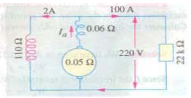
The drop in the series winding is \(102 \times 0.06 = 6.12\ \text{V}\), which with the armature drop sets the generated e.m.f.
One copper-loss term per winding:
The shunt-field loss can equally be written \(V_tI_f = 220 \times 2 = 440\ \text{W}\) — the same number, since the field is across the terminals.
The stray loss is what the efficiency leaves over. The overall efficiency fixes the input:
The torque comes from the input, not the output. The prime mover has to supply the whole 25 kW at 1000 rpm:
Using the 22 kW output instead would give 210.1 N·m and understate the driving engine by 12%.
A 4-pole DC shunt generator delivers 20 A to a load of 10 Ω. The armature resistance is 0.5 Ω and the shunt field resistance is 50 Ω. Allowing a drop of 1 V per brush, calculate the induced e.m.f. and the efficiency of the machine.
The load fixes the terminal voltage, which is the quantity the field winding sees:
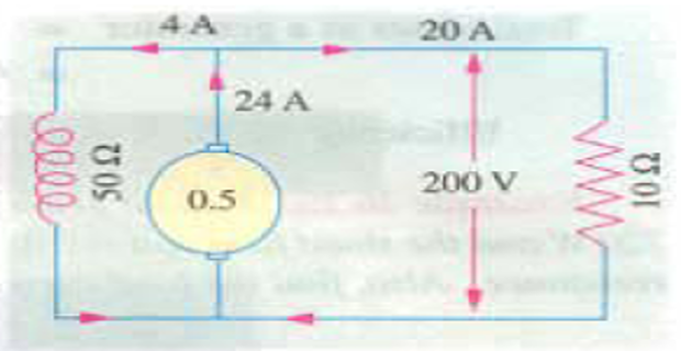
Field and armature currents:
Add every drop between the conductors and the terminals. There are two brushes in the circuit, one per polarity, so the contact drop is counted twice:
Only the electrical efficiency can be found, because no iron or friction loss is given — and without it the mechanical input is unknown:
Low, because this is a small machine: the 12 V armature drop is 6% of 200 V, where Problem 1's was 1.6%.
Where the missing 1136 W goes, as a check on the figure:
| Term | Value |
|---|---|
| Armature copper loss \(I_a^2R_a\) | \(24^2 \times 0.5 = 288\) W |
| Brush contact loss \(V_{\text{brush}}I_a\) | \(2 \times 24 = 48\) W |
| Shunt field loss \(V_tI_f\) | \(200 \times 4 = 800\) W |
| Total | 1136 W \(= 5136 - 4000\ \checkmark\) |
The field takes 800 W to deliver 4000 W — a 20% excitation burden that only a small machine would tolerate.
A long-shunt compound-wound generator gives 240 V at a full-load output of 100 A. The winding resistances are: armature (including brush contact) 0.1 Ω, series field 0.02 Ω, interpole field 0.025 Ω, and shunt field including its regulating resistance 100 Ω. The iron loss at full load is 1000 W and the windage and friction losses total 500 W. Calculate the full-load efficiency of the machine.
Collect the resistances that carry the armature current into a single armature-circuit resistance. The armature, series field and interpole field are all in the same series path:
The shunt field is not in this path — it is across the terminals and is treated separately.
The currents, with the long-shunt connection again putting \(I_a\) through the series and interpole windings:
The loss ledger:
The efficiency, with the input formed by adding the losses to the known output:
Roughly 42% of the loss is armature-circuit copper and varies with the square of the load; the other 58% — field copper, iron, windage and friction — is fixed. That split is what makes the maximum-efficiency point of Problem 2 fall well below full load.
A 250 V DC shunt machine is run light as a motor for a Swinburne's test and takes 5 A from the supply at no load. The armature resistance is 0.4 Ω and the shunt field resistance is 125 Ω. Determine the efficiency of the machine
- when running as a motor taking 50 A from the 250 V mains
- when running as a generator delivering 50 A at 250 V.
The point of the no-load run is to measure everything that will not change when the machine is loaded. At no load the machine develops almost no torque, so the whole input goes into losses:
Subtract the one loss that is load-dependent — the no-load armature copper loss — and what remains is the constant loss:
This 1246.4 W contains the shunt field loss \(250 \times 2 = 500\ \text{W}\) together with 746.4 W of iron, friction and windage loss. It stays the same at every load and in either mode of operation.
aAs a motor taking 50 A. The field still draws 2 A, so the armature takes the rest:
bAs a generator delivering 50 A. Now the armature must supply the field as well as the load, so the armature current is larger and the copper loss higher:
Why the generator figure is the higher of the two, despite its larger copper loss. In the motor the 50 A is the input and the losses are subtracted from it; in the generator the 50 A is the output and the losses are added to it. The same loss therefore appears against a larger denominator:
| Quantity | As motor | As generator |
|---|---|---|
| \(I_a\) | 48 A | 52 A |
| Armature copper loss | 921.6 W | 1081.6 W |
| Constant loss | 1246.4 W | 1246.4 W |
| Input | 12,500 W | 14,828 W |
| Efficiency | 82.66% | 84.30% |
What the test cannot tell you. The machine was never loaded, so the iron loss is measured at no-load flux rather than at the flux the load produces, stray load loss is missed entirely, and nothing at all is learnt about commutation or temperature rise. Swinburne's test is a prediction, not a demonstration — which is exactly the gap Problem 7 closes.
A Hopkinson's test on two identical 250 V DC shunt machines, mechanically coupled and electrically connected back to back, gave the following readings:
- current drawn from the supply into the two armature circuits, excluding the field currents: 25 A
- armature current of the machine acting as generator: 200 A
- field currents: 3 A for the generator, 2.5 A for the motor
- armature resistance of each machine: 0.02 Ω
Assuming the stray losses are equal in the two machines, calculate the efficiency of each.
Find the two armature currents first. The generator armature feeds the motor armature directly; the supply makes up only the shortfall, so at the junction
The motor must carry more current than the generator delivers, because it has to make good the losses of both machines.
The supply pays for the losses and nothing else. The power drawn into the armature circuits is therefore the total armature-circuit loss of the pair:
The stray loss is the remainder, shared equally between two machines assumed identical and running at the same speed and flux:
This covers iron, friction and windage. The field copper losses are not in it, because the field currents were excluded from the 25 A reading.
Motor efficiency. Its input is everything the supply and the generator push into it — armature and field alike:
Generator efficiency. Its output is the armature power it delivers; its input is the shaft power plus its own excitation:
Check the shaft. The two machines are bolted together, so the motor's mechanical output must be the generator's mechanical input — and the generator's input above includes 750 W of electrical excitation that never crosses the coupling:
A second check: the total supplied power \(250(25 + 3 + 2.5) = 7625\ \text{W}\) equals the sum of all six loss terms, \(1012.5 + 800 + 625 + 750 + 4437.5\).
Why the test is worth the trouble. Two 50 kW machines have been run at full load and full temperature on a supply of 7.6 kW, under 8% of the 100 kW the pair is handling. Nothing is dissipated in a load bank, the machines can be left running for a heat run, and the losses are measured at true load flux rather than extrapolated from no load.
| Loss term | Motor | Generator |
|---|---|---|
| Armature copper | 1012.5 W | 800 W |
| Field copper | 625 W | 750 W |
| Stray (half each) | 2218.75 W | 2218.75 W |
| Total | 3856.25 W | 3768.75 W |
| Efficiency | 93.22% | 92.99% |
Key Formulas
| Quantity | Relation | Notes |
|---|---|---|
| Shunt generator currents | \(I_a = I_L + I_f,\ \ I_f = V_t/R_{sh}\) | Armature feeds load and field — Problems 1, 4 |
| Generated e.m.f. | \(E_a = V_t + I_a(R_a+R_{se}) + V_{\text{brush}}\) | Long shunt; drop the \(R_{se}\) term for a plain shunt machine |
| Armature copper loss | \(P_{cu,a} = I_a^2R_a\) | Variable; scales as the square of load |
| Shunt field copper loss | \(P_{cu,f} = V_tI_f = I_f^2R_{sh}\) | Constant — Problems 1, 3, 5 |
| Brush contact loss | \(P_{\text{brush}} = V_{\text{brush}}I_a\) | Fixed volts per brush, so loss is linear in \(I_a\) — Problem 4 |
| Power developed in armature | \(P_d = E_aI_a\) | The mechanical/electrical hinge — Problem 1 |
| Mechanical efficiency | \(\eta_m = E_aI_a/P_{\text{mech,in}}\) | Excludes iron and friction only |
| Electrical efficiency | \(\eta_e = V_tI_L/E_aI_a\) | Excludes copper only |
| Commercial efficiency | \(\eta_c = V_tI_L/P_{\text{mech,in}} = \eta_m\eta_e\) | The overall figure — Problems 1, 3, 5 |
| Maximum efficiency | \(I_a^2R_a = P_{\text{const}}\) | Variable loss equals constant loss — Problem 2 |
| Prime-mover torque | \(T = 60P_{\text{mech,in}}/2\pi N\) | Uses the input, never the output — Problem 3 |
| Swinburne constant loss | \(P_{\text{const}} = V_tI_0 - I_{a0}^2R_a\) | Includes the field loss — Problem 6 |
| Swinburne efficiency (motor) | \(\eta = \dfrac{V_tI_L - I_a^2R_a - P_{\text{const}}}{V_tI_L}\) | \(I_a = I_L - I_f\) — Problem 6 |
| Swinburne efficiency (generator) | \(\eta = \dfrac{V_tI_L}{V_tI_L + I_a^2R_a + P_{\text{const}}}\) | \(I_a = I_L + I_f\) — Problem 6 |
| Hopkinson stray loss | \(P_{\text{stray}} = \tfrac12\left[V_tI_1 - I_{a,m}^2R_a - I_{a,g}^2R_a\right]\) | \(I_1\) is the armature-circuit supply current — Problem 7 |
Common Mistakes
Using the load current in \(I_a^2R_a\). The armature carries the field current too, so a generator's armature current is \(I_L + I_f\), not \(I_L\) — Problems 1 and 5, where 195 A becomes 200 A and 100 A becomes 102.4 A.
Confusing the three efficiencies. Mechanical, electrical and commercial differ only in where the boundary is drawn; quoting \(\eta_e\) when the question asks for the overall figure overstates it by four points — Problem 1.
Computing the prime-mover torque from the output. The shaft carries the input power, which includes every loss in the machine — Problem 3, where the error would be 12%.
Putting the load current through the series field of a long-shunt machine. Long shunt means the shunt field is outside the series winding, so the series field carries \(I_a\) — Problems 3 and 5.
Folding the brush drop into \(R_a\). It is a roughly constant voltage, counted once per brush, so two brushes give 2 V regardless of current — Problem 4.
Assuming maximum efficiency occurs at full load. It occurs where the variable loss equals the constant loss, here at 60% of full load — Problem 2.
Leaving the shunt field loss out of the Swinburne constant loss. The no-load input already contains it; subtracting only the armature copper loss keeps it where it belongs — Problem 6.
Using the same armature current for motor and generator operation. At the same 50 A terminal current the armature carries 48 A as a motor and 52 A as a generator — Problem 6.
Treating the Hopkinson supply current as the machine's input. It supplies the losses only; the motor's input is \(V_t(I_{a,m}+I_{f,m})\) — Problem 7.
Forgetting that field currents are excluded from the stray-loss balance. Field copper loss is charged to each machine separately, not split — Problem 7.
The DC machine is now complete as an engineering object. Sets 9 to 13 described what it does; this set describes what it costs, and the two testing methods show how that cost is measured on a machine too large to load directly. The loss ledger — variable copper against constant iron, friction and excitation — is not a DC idea at all, and neither is the maximum-efficiency condition that falls out of it.
Remove the commutator and the shaft, and what is left is two windings sharing an iron core. The same losses reappear under the same names, the same open-circuit and short-circuit tests separate them, and the same condition fixes the load of maximum efficiency. What changes is that the flux now alternates, and an e.m.f. equation must be written for it before anything else can be said.
Next: Set 15 — Transformer Fundamentals and the EMF Equation, where \(E = 4.44fN\Phi_m\) is used to size a core, count turns and find the flux density that everything else depends on.