By the end of this chapter you should be able to:
Define the hysteretic angle of advance and distinguish it from \(\phi_0\).
Explain the sequence by which the counterbalancing current appears.
Transfer resistance and reactance from one winding to the other.
Draw and use the exact equivalent circuit.
Derive the approximate equivalent circuit and state what it costs.
List the losses and identify which are constant and which vary.
Compute efficiency at any load and locate the maximum.
Compute all-day efficiency and explain why it differs.
Case 1 — Transformer on No Load
Even under no load, \(I_0\) is not wholly reactive. It has a small in-phase component supplying the iron loss.
\(I_0\) is small — 2 to 6 % of the full-load primary current in a power transformer, and as little as 1 % in very large units.
Because \(I_0\) is small, the no-load primary copper loss is negligible, so the no-load primary input is practically equal to the iron loss.
Since the core permeability varies with the instantaneous value of \(I_\mu\), the wave of \(I_\mu\) is not truly sinusoidal. Strictly it should not be drawn as a phasor — only sinusoids may be — but using its equivalent sine wave makes no practical difference.
It is the core loss that shifts the current vector. Without it, \(I_0\) would be purely magnetising and exactly in phase with the flux. The hysteresis loss pulls it forward.
\(\alpha\) is the angle by which \(I_0\) leads the flux, and it is this angle — not \(\phi_0\) — that is called the hysteretic angle of advance.
The distinction matters: \(\phi_0\) is measured from \(V_1\) and is large (about 80°); \(\alpha\) is measured from \(\Phi\) and is small (about 10°). They are complementary, and confusing them inverts the physics — a bigger core loss makes \(\alpha\) larger but \(\phi_0\) smaller.
Problem. The 2200/220 V, 50 kVA transformer of Chapters 41–43 has \(I_0 = 1.2\) A at \(\cos\phi_0 = 0.1894\). Find the hysteretic angle of advance, and verify it from the current components.
From the power factor.
Verification from the components. Since \(I_\mu\) is in phase with \(\Phi\) and \(I_w\) is perpendicular to it:
Comment. Note the direction of the dependence. A lossier core gives a larger \(I_w\), hence a larger \(\alpha\) and a smaller \(\phi_0\) — the current advances further ahead of the flux. A perfect, loss-free core would give \(\alpha = 0\) and \(\phi_0 = 90^{\circ}\), the ideal transformer of Chapter 41.
Ten degrees is typical. It is small because the iron loss is small compared with the reactive volt-amperes needed to magnetise the core.
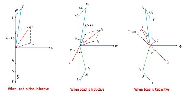
Case 2 — Transformer on Load
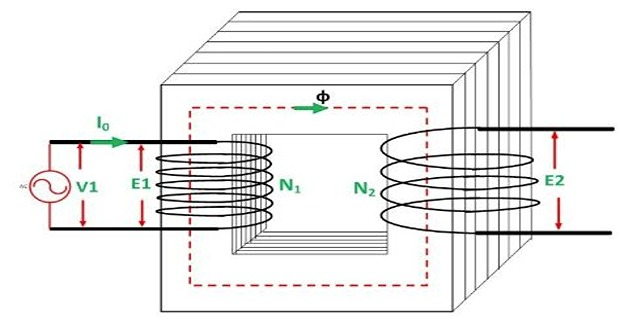
The secondary is connected to a load, which may be resistive, inductive or capacitive.
A current \(I_2\) flows through the secondary winding.
Its magnitude \(\left|I_2\right|\) depends on \(V_2\) and the load impedance.
The phase angle between \(I_2\) and \(V_2\) depends on the nature of the load.
The Counterbalancing Current

The chain of cause and effect is worth following in order, because it explains why a transformer needs no control system to respond to load.
- With the secondary open, the no-load current sets up the MMF \(N_1I_0\), which establishes the flux \(\Phi\) in the core.
- When load is connected, \(I_2\) flows and produces its own MMF \(N_2I_2\), setting up a flux \(\Phi_2\).
- By Lenz's law, \(\Phi_2\) opposes \(\Phi\). The resultant flux falls, and with it the induced EMF \(E_1\).
- Now \(V_1\) exceeds \(E_1\) by more than before, so an additional primary current \(I_1'\) is drawn from the supply.
- This additional current restores the original flux, so that \(V_1 = E_1\) again — hence the name primary counterbalancing current.
- \(I_1'\) is in phase opposition with \(I_2\). Its MMF \(N_1I_1'\) sets up \(\Phi_1'\), in the same direction as \(\Phi\), exactly cancelling \(\Phi_2\).
The flux is restored, so the iron loss and the magnetising current are unchanged by load — which is the assumption every efficiency calculation in this chapter relies on.
The steps 2 to 5 describe a transient that in practice is over in a fraction of a cycle. In the steady state the flux never actually changes; the description is a way of seeing why the primary current must follow the secondary.
Winding Resistance and Its Transfer
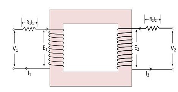
In an actual transformer there is resistance in both windings, because both are wound with copper. Taking resistance alone, with no leakage:
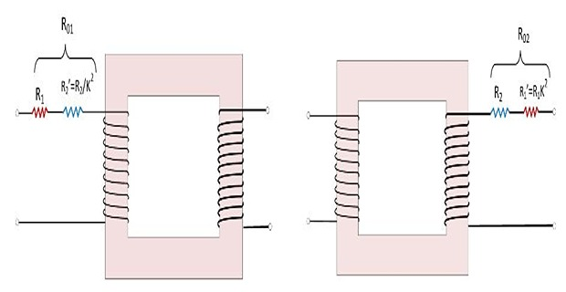
The resistance of the two windings can be transferred to either one winding. The advantage is that all calculations are then done in a single circuit.
The equivalent secondary resistance referred to the primary is the resistance which, carrying \(I_1\), would cause the same loss:
using \(I_2/I_1 = 1/K\) and neglecting \(I_0\). Similarly the primary resistance referred to the secondary is

Leakage Flux and Reactance
It is impossible to link all the flux with both \(N_1\) and \(N_2\).
Part of the flux linked with \(N_1\) — call it \(\Phi_{L_1}\) — does not link \(N_2\), completing its magnetic circuit through air rather than through the core.
The primary leakage flux is produced by the primary ampere-turns. \(\Phi_{L_1}\) is in phase with \(I_1\) and induces \(e_{L_1}\) in the primary but not in the secondary.
The same applies to the secondary leakage flux \(\Phi_{L_2}\).
At no load or light load the ampere-turns are small, so the leakage fluxes are negligible.
As load increases, both windings carry large currents generating large MMF, so there is appreciable leakage flux.
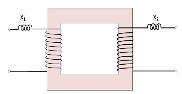
Reactances transfer by the same square law as resistances, since the criterion is again equal reactive volt-amperes:
The Exact Equivalent Circuit
Everything established so far can now be drawn as one circuit. Five parameters describe the transformer completely.
| Parameter | Represents | Measured by |
|---|---|---|
| \(R_{01}\) | Total winding resistance | Short-circuit test |
| \(X_{01}\) | Total leakage reactance | Short-circuit test |
| \(R_0\) | Iron loss | Open-circuit test |
| \(X_0\) | Magnetising reactance | Open-circuit test |
| \(K\) | Turns ratio | Voltage measurement |
Chapter 46 shows that two simple tests, neither requiring a load, yield all four impedances.
Referring the secondary to the primary means applying the rules of Chapter 41 to every secondary quantity at once:
Problem. Collect the parameters of the 2200/220 V, 50 kVA transformer from Chapters 42 and 43, and give the equivalent circuit referred to each side.
From Chapter 43 (winding quantities) and Chapter 42 (exciting branch):
Referred to the primary.
Referred to the secondary.
Comment. Note the enormous disparity of scale. The series impedance is 4.8 \(\Omega\) and the shunt branch about 1800 \(\Omega\) — a ratio of nearly 400 to 1. That disparity is exactly what makes the approximation of the next section so accurate.
A useful check: \(Z_{02}/Z_{01} = 0.04797/4.797 = 0.01 = K^{2}\) \(\checkmark\) Every impedance must scale by the same factor, so if any one does not, an arithmetic slip has occurred.
The Approximate Equivalent Circuit
The exact circuit is awkward: the exciting branch sits between the two series impedances, so the two cannot simply be added. Since \(I_0\) is only a few percent of \(I_1\), moving the exciting branch to the input terminals costs very little.
With the shunt branch at the terminals, the same current flows through all four series elements, so
a single equation replacing the two-stage calculation of Chapter 43. The exciting branch, now carrying \(V_1\) instead of \(E_1\), is simply a fixed load on the supply and plays no part in the series calculation at all.
The exciting branch now sees \(V_1\) rather than \(E_1\), so \(I_0\) comes out slightly too large, and \(I_1\) no longer flows through \(R_1\) and \(X_1\) — only \(I_2'\) does.
Both errors are of the order of \(I_0/I_1\), a few percent, and they act in opposite directions, so the net error is smaller still. Example 44.3 measures it.
Problem. Using the approximate circuit, find the primary voltage needed to hold 220 V at the secondary at full load, 0.8 lagging. Compare with the exact value of 2291.24 V found in Example 43.3.
Referred secondary voltage and current.
Applying the single equation.
Resolving the drop into components along and perpendicular to \(V_2'\):
Comparison.
Comment. The approximate circuit is low by 2.9 V in 2291 V — an error of one part in 800. For a calculation whose input data are rarely known to better than 1 %, this is entirely negligible, and the approximate circuit is what is used in practice throughout.
Note also the shape of the answer. The in-phase component of the drop is 87.4 V while the quadrature component is 65.1 V, yet the quadrature term contributes only \(\sqrt{2287.4^{2} + 65.1^{2}} - 2287.4 = 0.93\) V to the magnitude. The quadrature component of a small drop scarcely affects the length of a long phasor — the observation on which Chapter 45's approximate regulation formula rests.
Losses in a Transformer
Having no rotating parts, a transformer has only two kinds of loss — and Chapter 33's division into constant and variable applies unchanged.
| Loss | Where | Varies as | Measured by |
|---|---|---|---|
| Hysteresis | Core | \(B_m^{1.6}f\) — constant | Open-circuit test |
| Eddy current | Core | \(B_m^{2}f^{2}t^{2}\) — constant | |
| Primary copper | Winding | \(I_1^{2}R_1\) — as load² | Short-circuit test |
| Secondary copper | Winding | \(I_2^{2}R_2\) — as load² | |
| Stray load loss | Tank, clamps | as load² | Usually lumped with copper |
| Dielectric loss | Oil, insulation | Constant, very small | Neglected |
From Chapter 41, \(\Phi_m = V_1/4.44fN_1\) — no load current appears. The counterbalancing current of Section 44-3 restores the flux as fast as the load disturbs it.
So the iron loss can be measured with no load connected at all, and the copper loss with no voltage applied to speak of. That is the whole basis of the two tests of Chapter 46.
where \(x\) is the fraction of full load. Setting \(\mathrm{d}\eta/\mathrm{d}x = 0\) gives Chapter 33's condition again:
Problem. The transformer has an iron loss of 500 W. Using \(R_{02} = 0.01360~\Omega\), find the full-load copper loss and tabulate the efficiency at quarter, half, three-quarter, full and 125 % load at 0.8 power factor. Locate the maximum.
Full-load copper loss.
which agrees with the 702 W of Chapter 43, as it must \(\checkmark\)
| Load \(x\) | kVA | Output (W) | Copper (W) | Total loss (W) | Efficiency |
|---|---|---|---|---|---|
| 0.25 | 12.5 | 10 000 | 43.9 | 543.9 | 94.84 % |
| 0.50 | 25.0 | 20 000 | 175.6 | 675.6 | 96.73 % |
| 0.75 | 37.5 | 30 000 | 395.1 | 895.1 | 97.10 % |
| 0.844 | 42.2 | 33 750 | 500.0 | 1000.0 | 97.12 % |
| 1.00 | 50.0 | 40 000 | 702.5 | 1202.5 | 97.08 % |
| 1.25 | 62.5 | 50 000 | 1097.6 | 1597.6 | 96.90 % |
Location of the maximum.
Comment. The curve is remarkably flat near the top: from 75 % to 125 % of full load the efficiency varies only between 96.90 % and 97.12 %, a span of 0.22 percentage points. A transformer is essentially equally efficient over its whole useful range, which is why the exact location of the maximum is of little practical concern.
At light load, however, the picture changes sharply. At quarter load the efficiency has fallen to 94.84 %, because the constant 500 W iron loss is now being carried by only 10 kW of output. Transformers should not be left energised and lightly loaded, and this is exactly what the next example quantifies.
Commercial and All-Day Efficiency
The efficiency of Table 44.2 is the commercial or power efficiency — a ratio of powers at one instant. For a distribution transformer it is the wrong figure.
The distinction matters because a distribution transformer is energised 24 hours a day but loaded for only a few. The iron loss runs the whole time; the copper loss only when there is load.
All-day efficiency is therefore always lower than commercial efficiency, and is improved by designing for a low iron loss even at the cost of higher copper loss.
This is why a distribution transformer and a power transformer of the same rating are designed differently. A power transformer at a generating station runs near full load continuously, so it is designed for maximum efficiency at or near full load. A distribution transformer is designed with its maximum efficiency at perhaps half load, and with iron loss deliberately kept small.
Problem. The 50 kVA transformer supplies: full load at 0.8 power factor for 6 hours, half load at 0.9 power factor for 6 hours, and no load for the remaining 12 hours. Find its all-day efficiency and compare with the full-load commercial efficiency.
Output energy.
Copper-loss energy. Copper loss varies as \(x^{2}\):
Iron-loss energy. Constant for the whole 24 hours:
All-day efficiency.
Compare the commercial efficiency at full load from Table 44.2: \(97.08\,\%\).
Comment. The all-day figure is 1.48 percentage points lower. The reason is stark in the numbers: the iron loss contributes 12.00 kWh against the copper loss's 5.27 kWh — more than twice as much — because it runs for 24 hours while the copper loss runs for only 12, and at reduced load for half of those.
Note what would improve the figure. Halving the iron loss to 250 W would save 6 kWh a day and raise the all-day efficiency to 97.11 %... a gain of 1.5 points, whereas halving the copper loss would save only 2.6 kWh. For this duty cycle, iron loss is worth roughly twice as much attention as copper loss — and that is precisely how distribution transformers are designed.
Summary and Key Formulas
On no load \(I_0\) is not wholly reactive; the core loss advances it ahead of the flux by the hysteretic angle of advance \(\alpha = 90^{\circ} - \phi_0\).
On load, the secondary MMF opposes the flux; \(E_1\) falls; the primary draws a counterbalancing current \(I_1' = KI_2\) that restores it. Hence \(\overrightarrow{I_1} = \overrightarrow{I_0} + \overrightarrow{I_1'}\).
Resistance and reactance transfer by \(K^{2}\), the criterion being equal loss: \(R_2' = R_2/K^{2}\), \(R_1' = K^{2}R_1\).
Leakage flux links one winding only, completes its path through air, is in phase with its own current, and is negligible at light load.
The exact equivalent circuit has \(R_1\), \(X_1\) in series, then the exciting branch \(R_0 \parallel X_0\), then \(R_2'\), \(X_2'\).
The approximate circuit moves the exciting branch to the input, giving one series impedance \(R_{01} + jX_{01}\). The error is about 0.1 %.
Losses: iron (constant, since flux is fixed by the supply) and copper (varying as load²).
Maximum efficiency at \(x = \sqrt{P_i/P_{\text{Cu,FL}}}\), and the curve is very flat near the top.
All-day efficiency is a ratio of energies over 24 hours and is always lower, because iron loss runs continuously.
| Quantity | Formula | Notes |
|---|---|---|
| Hysteretic angle of advance | \(\alpha = 90^{\circ} - \phi_0\) | from the flux, not \(V_1\) |
| Counterbalancing current | \(I_1' = KI_2\) | antiphase with \(I_2\) |
| Primary current | \(\overrightarrow{I_1} = \overrightarrow{I_0} + \overrightarrow{I_1'}\) | phasor sum |
| Referred resistance | \(R_2' = R_2/K^{2}\) | equal-loss criterion |
| Equivalent resistance | \(R_{01} = R_1 + R_2/K^{2}\) | \(R_{02} = K^{2}R_{01}\) |
| Equivalent reactance | \(X_{01} = X_1 + X_2/K^{2}\) | \(X_{02} = K^{2}X_{01}\) |
| Approximate circuit | \(\mathbf{V}_1 = \mathbf{V}_2' + \mathbf{I}_2'\left(R_{01}+jX_{01}\right)\) | error ≈ 0.1 % |
| Copper loss | \(P_{\text{Cu}} = x^{2}I_2^{2}R_{02}\) | varies as load² |
| Efficiency | \(\eta = \dfrac{xS\cos\phi}{xS\cos\phi + P_i + x^{2}P_{\text{Cu,FL}}}\) | — |
| Maximum efficiency | \(x = \sqrt{P_i/P_{\text{Cu,FL}}}\) | variable = constant |
| All-day efficiency | \(\dfrac{\text{kWh out}}{\text{kWh out} + \text{kWh loss}}\) | over 24 h |
Common Mistakes
Calling \(\phi_0\) the hysteretic angle of advance. That is \(\alpha = 90^{\circ} - \phi_0\), measured from the flux.
Transferring impedance with \(K\) instead of \(K^{2}\). The criterion is equal \(I^{2}R\), so the square is unavoidable.
Multiplying when you should divide. Secondary to primary is \(\div K^{2}\); primary to secondary is \(\times K^{2}\).
Adding \(R_1\) and \(R_2'\) in the exact circuit. They are separated by the exciting branch and carry different currents.
Using \(I_1\) in the approximate circuit. The series drop is carried by \(I_2'\).
Letting the iron loss vary with load. The flux is fixed by the supply, so it does not.
Forgetting \(\cos\phi\) in the output. Efficiency uses kW, not kVA.
Using kVA in the all-day calculation. The numerator is energy, so the power factor must be applied at each stage.
Omitting the no-load hours from the iron-loss energy. It runs for the full 24 hours.
Expecting all-day efficiency to exceed commercial efficiency. It is always lower.
Chapter Review
Decide first which side you are working on, and refer every impedance to that side before starting.
P44.1 A transformer draws \(I_0 = 0.8\) A at a power factor of 0.25. Find \(\phi_0\) and the hysteretic angle of advance.
Show answer
Check: \(I_w = 0.200\) A, \(I_\mu = 0.7746\) A, \(\arctan(0.200/0.7746) = 14.48^{\circ}\) \(\checkmark\)\[\phi_0 = \arccos(0.25) = 75.52^{\circ}, \qquad \alpha = 90 - 75.52 = 14.48^{\circ}\]P44.2 A 1100/220 V transformer has \(R_1 = 0.5~\Omega\), \(R_2 = 0.02~\Omega\), \(X_1 = 1.6~\Omega\), \(X_2 = 0.064~\Omega\). Find \(R_{01}\), \(X_{01}\), \(R_{02}\), \(X_{02}\).
Show answer
\[K = 0.2, \quad K^{2} = 0.04\]\[R_{01} = 0.5 + \frac{0.02}{0.04} = 1.00~\Omega, \qquad X_{01} = 1.6 + \frac{0.064}{0.04} = 3.20~\Omega\]\[R_{02} = (0.04)(1.00) = 0.0400~\Omega, \qquad X_{02} = (0.04)(3.20) = 0.1280~\Omega\]P44.3 For P44.2, a 25 kVA rating gives \(I_2 = 113.6\) A. Find the full-load copper loss.
Show answer
\[P_{\text{Cu}} = I_2^{2}R_{02} = (113.6)^{2}(0.0400) = 516.2~\mathrm{W}\]P44.4 That transformer has an iron loss of 300 W. Find the efficiency at full load, 0.8 pf, and the load for maximum efficiency.
Show answer
\[\eta = \frac{(25\,000)(0.8)}{20\,000 + 300 + 516.2} = \frac{20\,000}{20\,816.2} = 96.08\,\%\]\[x = \sqrt{\frac{300}{516.2}} = 0.7624 \quad\Longrightarrow\quad 19.06~\mathrm{kVA}\]P44.5 For that transformer, find the maximum efficiency at 0.8 power factor.
Show answer
\[P_{\text{out}} = (19\,060)(0.8) = 15\,248~\mathrm{W}, \qquad \text{losses} = 2(300) = 600~\mathrm{W}\]Only 0.13 points above the full-load figure — the curve is flat.\[\eta_{\max} = \frac{15\,248}{15\,848} = 96.21\,\%\]P44.6 A 40 kVA transformer with 350 W iron loss and 600 W full-load copper loss runs at full load 0.8 pf for 4 h, half load 0.8 pf for 8 h, and no load for 12 h. Find the all-day efficiency.
Show answer
\[\text{output} = (40)(1.0)(0.8)(4) + (40)(0.5)(0.8)(8) = 128 + 128 = 256~\mathrm{kWh}\]\[\text{copper} = \frac{(600)(1)(4) + (600)(0.25)(8)}{1000} = 2.40 + 1.20 = 3.60~\mathrm{kWh}\]\[\text{iron} = \frac{(350)(24)}{1000} = 8.40~\mathrm{kWh}\]\[\eta_{\text{all-day}} = \frac{256}{256 + 3.60 + 8.40} = \frac{256}{268.0} = 95.52\,\%\]P44.7 Explain the sequence by which the primary current rises when load is applied.
Show answer
When load is connected, \(I_2\) flows and produces MMF \(N_2I_2\), setting up a flux \(\Phi_2\) which by Lenz's law opposes the main flux \(\Phi\).The resultant flux momentarily falls, so \(E_1\) falls. Since \(V_1\) is fixed, the difference \(V_1 - E_1\) increases, and an additional primary current \(I_1'\) is drawn.
\(I_1'\) is in phase opposition to \(I_2\), so its flux \(\Phi_1'\) is in the same direction as \(\Phi\) and exactly cancels \(\Phi_2\). The flux is restored, \(E_1\) returns to its original value, and equilibrium is reached with \(N_1I_1' = N_2I_2\).
The whole sequence is over in a fraction of a cycle; in the steady state the flux never actually changes. The description explains why the primary must follow the secondary, with no control system needed.
P44.8 Why does moving the exciting branch to the input terminals cause so little error?
Show answer
Because the exciting current is a very small fraction of the total. In the exact circuit \(I_0\) flows through \(R_1\) and \(X_1\) along with \(I_2'\); in the approximate circuit it does not. The omitted drop is \(I_0Z_1\), and with \(I_0\) at about 5 % of \(I_1\) this is a few tenths of a percent of the total.A second, opposing error appears: the exciting branch now sees \(V_1\) rather than the slightly smaller \(E_1\), so \(I_0\) comes out a little too large. The two errors act in opposite directions and partly cancel.
Example 44.3 measured the net effect as 0.125 % — negligible against data rarely known to better than 1 %.
P44.9 Why is all-day efficiency always lower than commercial efficiency, and how is it improved?
Show answer
Because the iron loss runs for all 24 hours whether or not the transformer is loaded, while the output energy accumulates only during the loaded hours. The denominator therefore carries a full day of iron loss against a partial day of output.To improve it, design for low iron loss, even at the cost of higher copper loss: better core steel, thinner laminations, and a lower working flux density (hence a larger core).
The consequence is that the maximum efficiency is placed at perhaps half load rather than full load, since \(x = \sqrt{P_i/P_{\text{Cu,FL}}}\) falls as \(P_i\) falls. This is exactly how distribution transformers differ from power transformers, which run near full load continuously and are optimised there.
P44.10 Why can the iron loss be measured at no load and the copper loss at negligible voltage?
Show answer
Iron loss at no load: the flux is set by \(\Phi_m = V_1/4.44fN_1\) and does not involve the load current. The counterbalancing current restores the flux as fast as the load disturbs it, so the flux — and hence the iron loss — is the same at any load. Applying rated voltage with the secondary open therefore gives the true iron loss, and the copper loss is negligible because \(I_0\) is only a few percent of rated current.Copper loss at low voltage: with the secondary short-circuited, rated current flows at only about 5 % of rated voltage. The flux is then 5 % of normal, so the iron loss is roughly \((0.05)^{1.6}\) to \((0.05)^{2}\) of its rated value — a fraction of a percent, entirely negligible. The wattmeter therefore reads copper loss alone.
Each test isolates one loss by making the other negligible, which is the basis of Chapter 46.
MCQ 1. The hysteretic angle of advance is measured from:
(a) \(V_1\) (b) the flux (c) \(E_2\) (d) \(I_2\)Show answer
(b) the flux. It equals \(90^{\circ} - \phi_0\).MCQ 2. The counterbalancing current \(I_1'\) is:
(a) in phase with \(I_2\) (b) in phase opposition to \(I_2\) (c) 90° from \(I_2\) (d) equal to \(I_0\)Show answer
(b) in phase opposition to \(I_2\), so that its flux cancels \(\Phi_2\).MCQ 3. The secondary resistance referred to the primary is:
(a) \(KR_2\) (b) \(R_2/K\) (c) \(K^{2}R_2\) (d) \(R_2/K^{2}\)Show answer
(d) \(R_2/K^{2}\), from equating the copper losses.MCQ 4. Leakage flux is in phase with:
(a) the main flux (b) its own winding current (c) the applied voltage (d) the induced EMFShow answer
(b) its own winding current, because its path is through air.MCQ 5. In the exact equivalent circuit, the exciting branch is placed:
(a) at the input terminals (b) after the primary impedance (c) at the output (d) in seriesShow answer
(b) after the primary impedance, since it is driven by \(E_1\), not \(V_1\).MCQ 6. The approximate equivalent circuit is useful because it:
(a) is more accurate (b) lets the series impedances be added (c) removes the iron loss (d) removes the turns ratioShow answer
(b) lets the series impedances be added into one \(R_{01} + jX_{01}\).MCQ 7. The iron loss of a transformer:
(a) varies as load (b) varies as load² (c) is constant (d) is zero at no loadShow answer
(c) is constant, because the flux is fixed by the supply.MCQ 8. Maximum efficiency occurs when:
(a) copper loss = iron loss (b) copper loss = 2 × iron loss (c) at full load always (d) at no loadShow answer
(a) copper loss = iron loss, i.e. variable loss equals constant loss.MCQ 9. All-day efficiency is:
(a) higher than commercial (b) lower than commercial (c) equal (d) undefinedShow answer
(b) lower, since iron loss runs for 24 hours regardless of load.MCQ 10. A distribution transformer is designed with:
(a) high iron loss (b) low iron loss (c) zero copper loss (d) maximum efficiency at full loadShow answer
(b) low iron loss, because it is energised continuously but loaded only part of the time.
Explain why \(I_0\) is not wholly reactive, and define the hysteretic angle of advance.
Trace the sequence by which the counterbalancing current appears when load is applied.
Derive the transfer of resistance from secondary to primary, stating the criterion used.
Explain what leakage flux is and why it varies with load.
Draw the exact equivalent circuit and identify each element.
Derive the approximate equivalent circuit and justify the approximation.
List the losses, stating which are constant and which vary, and why.
Distinguish commercial from all-day efficiency and explain the design consequence.
The equivalent circuit is complete, and Example 44.3 has already produced the quantity Chapter 45 is about. Holding 220 V at the secondary under full load at 0.8 lagging required 2288 V at the primary rather than 2200 V — so if 2200 V is applied instead, the secondary must fall below 220 V. That fall is the voltage regulation.
Chapter 45 defines it, derives the approximate formula
and shows why the quadrature term of Example 44.3 — which contributed only 0.93 V to a 2288 V phasor — may be dropped. It also derives the power factor of zero regulation and that of maximum regulation, which turn out to be at right angles to each other.
Chapter 46 then closes the loop by showing how \(R_{01}\), \(X_{01}\), \(R_0\) and \(X_0\) are all obtained from the open-circuit and short-circuit tests — for which P44.10 has already given the justification.