Excitation Impact: Synchronous Motor Current & Power Factor

Demonstrative Video

Effect of Excitation on Armature Current & PF

What happens under over excitation and under-excitation?
Consider SM having constant mechanical load (output constant, if losses neglected)

Case-1: $E_b = V$ known as 100% excitation
- armature $I$ lags $V$ by small angle $\phi$
- $\theta$ with $E_R$ is fixed by stator constants i.e. $\tan\theta=X_s/R_a$

Case-2: $E_b < V$ excitation is less than 100%
- $E_{R}$ advanced clockwise and so is $I$ (because it lags behind $E_{R}$ by fixed angle $\theta$ ).
- $|I|$ is increased but its PF is decreased ( $\phi$ has increased).
- Because input as well as $V$ are constant, hence the power component of $I$ i.e., $I \cos \phi$ remains same, but watt-less component $I$ $\sin \phi$ is increased.
- Hence, as excitation $\downarrow$ , $I~\uparrow$ but p.f. $\downarrow$ so that power component $I \cos \phi=OA$ remain constant.
- Locus of extremity of current vector is a straight horizontal line
- Incidentally, when $I_f~\downarrow$ , the pull-out torque is also $\downarrow$ in proportion.

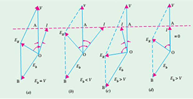
Case-3: $E_b > V$
- $E_{R}$ is pulled anticlockwise and so is $I$ .
- Now motor is drawing a leading current.
- For some value of excitation, that $I$ may be in phase with V i.e., p.f. is unity
- At that time, the current drawn by the motor would be minimum.

Two important points stand out clearly from the prevailing discussion:

$I_a$ Vs $I_f$
- $|I|$ varies with excitation and has large value both for low and high values of excitation (though it is lagging for low excitation and leading for higher excitation).
- In between, it has minimum value corresponding to a certain excitation.
- The variations of $I$ with excitation is known as V-curves because of their shape.

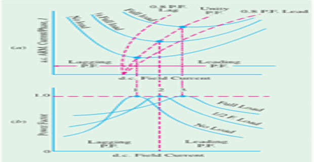
$\cos\phi$ Vs $I_f$
- For the same input, $I$ varies over a wide range and so causes the power factor also to vary accordingly.
- When over-excited, motor runs with leading p.f. and with lagging p.f. when under-excited. In between, the p.f. is unity.
- The variations of $p . f$ . with excitation looks like inverted V-curve.