By the end of this chapter you should be able to:
Set out the ampere-turn method as a repeatable procedure and apply it to any composite core.
Analyse a series magnetic circuit made of several materials and cross-sections, recognising that the flux is common and the mmfs add.
Handle an air gap as one more series section, and predict before calculating that it will dominate the mmf.
Analyse a parallel circuit in which flux divides between limbs sharing a common mmf, using permeances.
Solve a series–parallel circuit, computing both the total mmf and the division of flux between branches.
State the two magnetic Kirchhoff laws and use them to write the governing equations of any core.
Distinguish the direct problem (flux given, find mmf — one pass) from the inverse problem (mmf given, find flux — iterative when the iron is non-linear).
Compute the air gap required to achieve a specified flux for a given excitation.
Introduction
Chapter 2 dealt with the simplest possible magnetic circuit: one uniform path, one material, one cross-section. No real device looks like that. A transformer core has a central limb whose flux divides between two outer limbs. A machine's flux crosses from stator teeth, through an air gap, into rotor teeth, and returns through two yokes. A relay has a variable gap in series with a fixed iron path.
What makes these tractable is the observation from Section 2-6: since \(\Phi = \mathcal{F}/S\) has the same form as \(I = V/R\), every series–parallel technique from resistive circuit theory carries over unchanged. Reluctances in series add. Permeances in parallel add. Flux divides between parallel branches inversely as their reluctances, exactly as current does. Both Kirchhoff laws have magnetic counterparts.
This chapter turns that correspondence into a working method. The core skill is not conceptual difficulty but bookkeeping discipline: identifying the sections, computing \(B\) in each from the flux it carries, converting to \(H\) using the right permeability, and summing the \(Hl\) products around the correct loop. Students lose marks here through disorganisation far more often than through misunderstanding, so the procedure below is worth following literally until it becomes automatic.
The Ampere-Turn Method
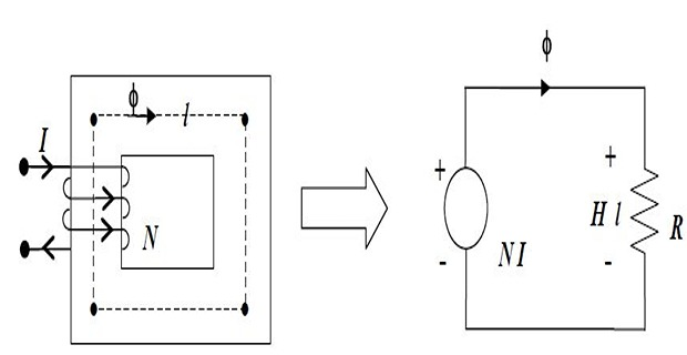
Start from Hopkinson's law and rearrange it to make the excitation the subject. For a single uniform section,
so the ampere-turns required to drive a flux \(\Phi\) through that section are
The last form is the one to remember. The ampere-turns absorbed by any section equal the field intensity in that section multiplied by its length. This is the magnetic counterpart of "volts dropped equal current times resistance", and it is what makes composite circuits easy: each section is handled separately, and the results are added.
Work section by section. For each, find the flux it carries, divide by its area to get \(B\), divide by its own permeability to get \(H\), multiply by its own length to get its ampere-turn drop. Then add the drops around one closed path. That is the entire method.
- Divide the core into sections. A new section begins wherever the material changes, the cross-section changes, or an air gap occurs.
- Find the flux in each section. In a series circuit this is the same throughout. Where the core branches, apply \(\sum\Phi = 0\) at the junction.
- Compute \(B_k = \Phi_k / A_k\) for each section, using that section's own area.
- Convert to \(H_k\) — by \(H = B/\mu_0\mu_r\) if a permeability is given, or by reading the B–H curve if one is supplied (Chapter 5). For an air gap, \(H_g = B/\mu_0\).
- Compute the drop \(H_k l_k\) for each section, taking care to use mean path lengths.
- Sum the drops around a closed loop to get the total mmf, then divide by \(N\) for the current.
Series Magnetic Circuits
A series magnetic circuit is one in which the whole of the flux passes through every section in turn. The defining features mirror the electrical case exactly:
The flux is common to all sections — \(\Phi_1 = \Phi_2 = \cdots = \Phi\).
The mmf drops add — \(NI = H_1l_1 + H_2l_2 + \cdots\).
The reluctances add — \(S_{eq} = S_1 + S_2 + \cdots\).
Note carefully that although the flux is common, the flux density generally is not: wherever the cross-section changes, \(B = \Phi/A\) changes with it. A narrow section carries the same flux crowded into less area, so it runs at higher \(B\) — and is therefore the section that saturates first. Identifying that section is often the whole point of a design calculation.
Problem. A closed magnetic circuit consists of two sections in series. Section 1 is wrought iron of length 0.30 m, cross-section 6 cm² and \(\mu_r = 2000\). Section 2 is cast steel of length 0.20 m, cross-section 4 cm² and \(\mu_r = 1000\). A coil of 500 turns is wound on the circuit. Find the current needed to establish a flux of 0.5 mWb, and identify which section is closer to saturation.
Section 1 — wrought iron.
Section 2 — cast steel.
Total.
Check by the reluctance route.
Which section saturates first? Section 2, at 1.25 T against Section 1's 0.83 T. Two independent factors work against it — it has the smaller area (so higher \(B\) for the same flux) and the poorer material (so higher \(H\) for that \(B\)). Between them these give it two-thirds of the total ampere-turns from less than half the path length. In any composite circuit, look first at the section with the smallest area and the worst material — it will dominate the answer.
Series Circuits with an Air Gap
An air gap is simply one more section in series, and it is handled by exactly the same procedure. The only difference — and it is the difference that matters — is that its permeability is \(\mu_0\), with no \(\mu_r\) multiplier.
Since the iron and the gap carry the same flux, and (neglecting fringing) have the same cross-section, they run at the same flux density \(B\). Their field intensities, however, differ by the factor \(\mu_r\):
The field intensity in the gap is thousands of times that in the iron, at the same flux density. Since the permeabilities of iron and air differ so greatly, the corresponding values of \(H\) — and therefore the ampere-turns absorbed per metre — are utterly different in the two media. The total flux follows as

Problem. A cast-steel ring has a mean circumference of 0.50 m and a uniform cross-section of 5 cm², with \(\mu_r = 1200\). A radial air gap of 1.5 mm is cut in it, and a coil of 600 turns is wound on the ring. Find the current required to produce a flux of 0.55 mWb, and the percentage of the mmf absorbed by the gap. Neglect fringing and leakage.
Flux density (common to iron and gap):
Iron section. The iron path is shortened by the gap:
Air gap. No \(\mu_r\):
Total.
MMF split.
Comment. The predicted ratio was \(S_g/S_i = (0.0015/0.4985)(1200) = 3.61\), giving \(3.61/4.61 = 78.3\,\%\) — exactly what the full calculation returned. Getting into the habit of making that one-line estimate first will catch most gap-related slips before they propagate.
Parallel Magnetic Circuits
A parallel magnetic circuit is one in which the flux divides between two or more paths that share a common mmf. The three-limb transformer core is the standard example: a coil on the central limb drives flux that splits at the top yoke, travels down the two outer limbs, and recombines at the bottom.
Two rules govern the junction, and both are the magnetic counterparts of Kirchhoff's laws:
Flux entering a junction equals flux leaving it. This follows from \(\nabla\cdot\mathbf{B} = 0\) — there are no magnetic monopoles, so flux cannot accumulate anywhere.
The applied ampere-turns equal the sum of the ampere-turn drops around any closed magnetic path. Parallel branches between the same two junctions therefore have equal mmf drops.
The second rule gives the working relation for two parallel branches. Since both are driven across the same pair of junctions,
and combining with \(\Phi = \Phi_1 + \Phi_2\) gives the flux-divider rule:
Note the cross-over: branch 1's flux carries branch 2's reluctance in the numerator. The easier path takes more flux — exactly as the smaller resistance takes more current. Working in permeances avoids the reciprocals entirely, which is why they exist.
Problem. A three-limb core has a central limb of length 0.20 m and cross-section 10 cm², carrying a 400-turn coil. Each of the two identical outer paths (limb plus half of each yoke) has length 0.45 m and cross-section 5 cm². Take \(\mu_r = 1500\) throughout. Find the current required to establish 1.2 mWb in the central limb.
Flux division. The outer paths are identical, so by symmetry each carries half:
Central limb.
One outer path. Half the flux, but half the area too — so the same flux density:
Total. Go once around one closed loop — central limb plus one outer path. Do not add both outer paths:
Check by reluctances.
Comment. The most common error in parallel problems is adding both outer branches' drops to the central one, giving 700 AT here instead of 414. The mmf is the drop around a single closed loop; the second outer limb is an alternative route for the same journey, not an additional leg of it.
Series–Parallel Circuits
The general case combines both patterns: a section carrying the whole flux in series with a group of branches that share it. Machine cores are invariably of this type, and so is any three-limb core with an air gap in one limb only.
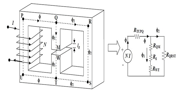

The governing equations follow directly from the two Kirchhoff analogues. With the total flux \(\Phi\) dividing into \(\Phi_1\) through a gapped branch and \(\Phi_2\) through a plain one:
The third line is the important one: the two parallel branches must absorb equal ampere-turns, because they connect the same two junctions. The fourth line is a consequence — once you know the drop across the parallel group (by whichever branch is easier to compute), you can ignore the other branch entirely when finding the total mmf.
For a series–parallel problem, the route depends on what you are given.
Given the total flux — compute both branch reluctances, use the divider rule to split the flux, then sum the series drop and either branch drop. This is Worked Example 3.4.
Given the flux in one branch — compute that branch's drop directly; that same drop applies to the other branch, so work backwards to get its flux; add the two to get the series flux; then compute the series drop. This is often the shorter route and is worth spotting.
Given the mmf — reduce the network to a single equivalent reluctance and divide. Straightforward only if the iron is linear; see Section 3-7.
Problem. A core has a central limb of length 0.25 m and cross-section 8 cm² carrying an 800-turn coil. The flux divides between two outer branches, each of iron length 0.40 m and cross-section 4 cm². One branch contains a 1 mm air gap. Take \(\mu_r = 1400\) for all iron and neglect fringing and leakage. For a total flux of 1.0 mWb in the central limb, find the current and the flux in each branch.
Step 1 — branch reluctances. With \(\mu = (4\pi\times10^{-7})(1400) = 1.7593\times10^{-3}\):
Step 2 — flux division. Flux divides inversely as reluctance:
Check: \(0.182 + 0.818 = 1.000\) mWb \(\checkmark\). The gapped branch takes only 18 % of the flux — the 1 mm of air makes that route four and a half times harder.
Step 3 — drop across the parallel group. Either branch will do; they must agree:
Step 4 — central limb and total.
Comment. Notice the design lesson hiding in the numbers. Cutting a 1 mm gap in one limb diverted 82 % of the flux into the other limb — a far larger effect than the 1.5 mm gap of Example 3.2 had on a series circuit. In a series circuit a gap costs you current; in a parallel circuit a gap costs you flux, because the flux simply goes elsewhere. This is precisely how a magnetic shunt works, and how flux is steered in ballasts and welding transformers.
The Direct and Inverse Problems
Every problem in this chapter is one of two kinds, and they are not equally difficult. Recognising which you face determines the method.
Given the flux, find the mmf.
Every step is a forward evaluation. Even with a non-linear B–H curve it is a single pass: you know \(B\), so you simply read \(H\) off the graph. All four worked examples so far are of this type.
Given the mmf, find the flux.
You cannot start, because \(H\) in each section depends on the flux you are trying to find. With constant \(\mu_r\) the chain closes algebraically. With a real B–H curve it does not, and the problem must be solved by iteration.
This asymmetry is worth dwelling on, because textbook problems are overwhelmingly of the easy kind while real design questions ("I have a 12 V supply and 800 turns — what flux do I get?") are overwhelmingly of the hard kind.
- Guess a flux \(\Phi^{(0)}\). A good opening guess ignores the iron entirely and treats the circuit as gap-only, since the gap usually dominates: \(\Phi^{(0)} \approx NI/S_g\). This always overestimates.
- Run the direct problem on that guess to find the mmf it would require, \(\mathcal{F}^{(0)}\).
- Compare with the mmf actually available. If \(\mathcal{F}^{(0)} > NI\) the guess was too high; reduce it, and conversely.
- Scale and repeat. A proportional correction \(\Phi^{(1)} = \Phi^{(0)}\left(NI/\mathcal{F}^{(0)}\right)\) converges quickly, because the relation is not far from linear below the knee. Two or three passes usually suffice.
A graphical alternative exists and is more elegant: plot the core's \(\Phi\)-versus-mmf characteristic and superimpose the straight "air-gap line" \(\Phi = (NI - \mathcal{F}_i)/S_g\). Their intersection is the operating point, found in one step with no iteration at all. Chapter 5 develops this construction properly once the B–H curve is available; Chapter 9 uses the same idea to locate the operating point of a permanent magnet.
Problem. The gapped ring of Worked Example 3.2 (iron path 0.4985 m, area 5 cm², \(\mu_r = 1200\), gap 1.5 mm, 600 turns) is supplied with 2.0 A. Find the resulting flux and flux density.
Solution. Since \(\mu_r\) is constant, the circuit is linear and the reluctance route gives the answer directly.
Consistency check. Example 3.2 needed 2.794 A for 0.55 mWb. Here 2.0 A gives 0.394 mWb, and
The exact proportionality is the signature of a linear circuit, and it is also the warning. Had this been a real cast-steel ring at 1.1 T, the permeability at 0.787 T would have been rather higher than at 1.1 T, so the true flux at 2.0 A would exceed 0.394 mWb. The constant-\(\mu_r\) model is at its worst precisely when you extrapolate away from the point at which \(\mu_r\) was quoted.
Applications
The core of Section 3-5 is a single-phase shell-type transformer. Its central limb carries the windings and the full flux; the outer limbs return it. Because each outer limb carries only half the flux, it is built with half the area — which is why shell-type cores have that characteristic stepped profile.
Example 3.4 showed that a gapped parallel branch steals or sheds flux dramatically. Deliberately adding such a branch — a magnetic shunt — diverts flux away from the secondary, giving the high leakage reactance that a welding transformer or a fluorescent ballast needs to limit current.
The total ampere-turns per pole of a DC machine are the sum of drops across yoke, pole core, pole shoe, air gap, armature teeth and armature core — a six-section series circuit solved exactly by the method of Section 3-2. Chapter 28 does this calculation in full.
A relay's iron path is in series with a gap that closes as the armature moves. The inverse problem of Section 3-7 is what determines whether a given coil will actually pull the armature in from its fully open position — the hardest condition, since the gap reluctance is then largest.
A gapped reactor is designed backwards: the desired inductance fixes \(S = N^2/L\), and since the gap dominates, the gap length follows almost immediately as \(l_g \approx \mu_0 A S\). The iron is then checked as a small correction.
Modern design uses numerical field solvers, but a hand calculation by the ampere-turn method remains the standard sanity check on a simulation. An FE result that disagrees with a careful magnetic-circuit estimate by more than 10–20 % usually indicates a modelling error, not a subtle field effect.
Summary and Key Formulas
The ampere-turn method handles any composite core: split into sections, find each section's flux, then \(B\), then \(H\), then \(Hl\), and sum around one closed loop.
In a series circuit the flux is common and the drops add. The flux density is not common — it rises wherever the area falls, so the narrowest section saturates first.
An air gap is just another series section, but with \(\mu_r = 1\). At equal flux density, \(H_g/H_i = \mu_r\), so the gap normally absorbs most of the ampere-turns.
In a parallel circuit the mmf is common and the flux divides inversely as reluctance. Add permeances, not reluctances.
The two magnetic Kirchhoff laws are \(\sum\Phi = 0\) at a junction and \(\sum NI = \sum Hl\) around a loop.
For a series–parallel core, parallel branches absorb equal ampere-turns. Sum the series drop and one branch drop — never both.
A gap in a series path costs current; a gap in a parallel branch costs flux, which simply diverts to the easier route.
The direct problem (flux given) is a single forward pass. The inverse problem (mmf given) is algebraic only if the iron is linear, and otherwise needs iteration or a graphical construction.
| Feature | Series circuit | Parallel circuit |
|---|---|---|
| Common quantity | Flux \(\Phi\) | MMF drop \(\mathcal{F}\) |
| Divided quantity | MMF, among sections | Flux, among branches |
| Combination rule | \(S_{eq} = \sum S_k\) | \(P_{eq} = \sum P_k\) |
| Governing law | \(NI = \sum H_k l_k\) | \(\Phi = \sum \Phi_k\) |
| Divider rule | \(\mathcal{F}_k = \mathcal{F}\dfrac{S_k}{\sum S}\) | \(\Phi_1 = \Phi\dfrac{S_2}{S_1+S_2}\) |
| Effect of an air gap | Raises the current needed | Diverts flux to the other branch |
| Electrical counterpart | Resistors in series | Resistors in parallel |
| Quantity | Formula | Notes |
|---|---|---|
| Ampere-turns of a section | \(NI = \dfrac{\Phi l}{A\mu_0\mu_r} = Hl\) | the core relation of the method |
| Series total mmf | \(NI = \sum H_k l_k = \Phi\sum S_k\) | flux common |
| Series reluctance | \(S_{eq} = S_1 + S_2 + \cdots\) | including any gap |
| Gap field intensity | \(H_g = \dfrac{B}{\mu_0}\) | \(H_g/H_i = \mu_r\) at equal \(B\) |
| Flux continuity | \(\sum\Phi = 0\) at a junction | magnetic KCL |
| MMF balance | \(\sum NI = \sum Hl\) round a loop | magnetic KVL |
| Equal-branch drop | \(\Phi_1 S_1 = \Phi_2 S_2\) | parallel branches |
| Flux divider | \(\Phi_1 = \Phi\dfrac{S_2}{S_1+S_2}\) | note the cross-over |
| Parallel reluctance | \(S_{eq} = \dfrac{S_1 S_2}{S_1+S_2}\) | two branches |
| Symmetric branches | \(\Phi_1 = \Phi_2 = \Phi/2\) | no divider rule needed |
| Series–parallel mmf | \(NI = \Phi S_c + \Phi_1 S_1\) | one branch only |
| Iteration correction | \(\Phi^{(1)} = \Phi^{(0)}\dfrac{NI}{\mathcal{F}^{(0)}}\) | inverse problem |
Common Mistakes
Adding both parallel branches to the series drop. The mmf is the drop around one closed loop. In Worked Example 3.3 this error would give 700 AT instead of 414 — a 69 % overestimate.
Assuming \(B\) is the same throughout a series circuit. The flux is common; the density changes wherever the area does. Recompute \(B\) for every section.
Using one section's \(\mu_r\) for another. Each section has its own material. Tabulate the sections before starting, one row each for \(l\), \(A\), \(\mu_r\), \(\Phi\), \(B\), \(H\) and \(Hl\).
Getting the flux divider the wrong way round. Branch 1's flux carries \(S_2\) on top. The easier path takes more flux — check your answer against that intuition every time.
Adding reluctances in parallel. Add permeances, or use \(S_1S_2/(S_1+S_2)\). Simply summing them gives an answer larger than either branch alone, which is transparently absurd.
Forgetting that a gap makes its branch less attractive. Students often expect the gapped branch to carry more flux because "the gap is where the action is". It carries less — usually far less.
Not subtracting the gap from the iron path. Minor for a 1 mm gap in 500 mm, but the habit matters when gaps are large.
Attempting the inverse problem by direct substitution when the iron is non-linear. There is no closed form. Iterate, or use the air-gap-line construction.
Mixing mean path lengths with outer or inner dimensions. Always use the mean path — the centre line of the core — unless the problem states otherwise.
Applying the flux divider to a circuit that is not actually parallel. Two branches are in parallel only if they connect the same two junctions. Check the geometry before reaching for the formula.
Chapter Review
Tabulate the sections before calculating. Where a parallel group appears, check that both branches give the same ampere-turn drop — that single check catches most errors.
P3.1 A series circuit has section 1 of length 0.25 m, area 5 cm², \(\mu_r = 2500\), and section 2 of length 0.15 m, area 3 cm², \(\mu_r = 1200\). Find the current in a 300-turn coil to establish 0.4 mWb.
Show answer
Section 1: \(B_1 = 0.4\times10^{-3}/5\times10^{-4} = 0.800\) T, \(\mu_1 = 3.1416\times10^{-3}\)Section 2: \(B_2 = 0.4\times10^{-3}/3\times10^{-4} = 1.333\) T, \(\mu_2 = 1.5080\times10^{-3}\)\[H_1 = \frac{0.800}{3.1416\times10^{-3}} = 254.6~\mathrm{AT/m}, \qquad \mathcal{F}_1 = (254.6)(0.25) = 63.7~\mathrm{AT}\]\[H_2 = \frac{1.333}{1.5080\times10^{-3}} = 884.2~\mathrm{AT/m}, \qquad \mathcal{F}_2 = (884.2)(0.15) = 132.6~\mathrm{AT}\]Section 2 takes 68 % of the mmf from 37 % of the length — smaller area and poorer material together.\[NI = 63.7 + 132.6 = 196.3~\mathrm{AT} \quad\Longrightarrow\quad I = \frac{196.3}{300} = 0.654~\mathrm{A}\]P3.2 A ring of mean circumference 0.60 m and area 6 cm² has \(\mu_r = 1800\) and a 2 mm gap. Find the iron and gap reluctances, their ratio, and the total.
Show answer
\(\mu = (4\pi\times10^{-7})(1800) = 2.2619\times10^{-3}\), iron length \(= 0.598\) m\[S_i = \frac{0.598}{(2.2619\times10^{-3})(6\times10^{-4})} = 4.406\times10^{5}~\mathrm{AT/Wb}\]\[S_g = \frac{0.002}{(4\pi\times10^{-7})(6\times10^{-4})} = 2.653\times10^{6}~\mathrm{AT/Wb}\]Check against the shortcut: \((l_g/l_i)\mu_r = (0.002/0.598)(1800) = 6.02\) \(\checkmark\). The gap takes 86 % of the mmf.\[\frac{S_g}{S_i} = 6.02, \qquad S_{\text{total}} = 3.093\times10^{6}~\mathrm{AT/Wb}\]P3.3 A symmetric three-limb core carries 1.5 mWb in its central limb of area 12 cm². Each outer limb has area 6 cm². Find the flux and flux density in each limb.
Show answer
By symmetry each outer limb carries \(1.5/2 = 0.75\) mWb.Both run at the same density — which is exactly why the outer limbs are built with half the area. Equal \(B\) everywhere is the mark of an efficiently proportioned core.\[B_c = \frac{1.5\times10^{-3}}{12\times10^{-4}} = 1.25~\mathrm{T}, \qquad B_o = \frac{0.75\times10^{-3}}{6\times10^{-4}} = 1.25~\mathrm{T}\]P3.4 Two parallel branches have reluctances \(8\times10^{5}\) and \(4\times10^{5}\) AT/Wb, carrying a total of 1.2 mWb. Find the equivalent reluctance and the flux in each.
Show answer
\[S_{eq} = \frac{(8\times10^{5})(4\times10^{5})}{12\times10^{5}} = 2.667\times10^{5}~\mathrm{AT/Wb}\]Check the drops: \((4\times10^{-4})(8\times10^{5}) = 320\) AT and \((8\times10^{-4})(4\times10^{5}) = 320\) AT \(\checkmark\)\[\Phi_1 = 1.2\times\frac{4}{12} = 0.400~\mathrm{mWb}, \qquad \Phi_2 = 1.2\times\frac{8}{12} = 0.800~\mathrm{mWb}\]P3.5 In a parallel arrangement, branch 1 has \(H_1 = 400\) AT/m over 0.30 m. Branch 2 has length 0.24 m. What must \(H_2\) be, and why?
Show answer
Parallel branches connect the same two junctions, so they must absorb equal ampere-turns:The shorter branch needs a higher field intensity to absorb the same total drop — the magnetic KVL in one line.\[H_1l_1 = H_2l_2 \quad\Longrightarrow\quad H_2 = \frac{(400)(0.30)}{0.24} = 500~\mathrm{AT/m}\]P3.6 A core has a central limb of length 0.20 m, area 10 cm², and two outer branches each of iron length 0.50 m and area 5 cm². One outer branch contains a 0.5 mm gap. With \(\mu_r = 2000\) throughout and a 500-turn coil, find the current for a central flux of 1.4 mWb, and the flux in each branch.
Show answer
\(\mu = 2.5133\times10^{-3}\). Branch reluctances:\[S_A = \frac{0.4995}{1.2566\times10^{-6}} + \frac{0.0005}{6.2832\times10^{-10}} = 3.975\times10^{5} + 7.958\times10^{5} = 1.1933\times10^{6}\]\[S_B = \frac{0.500}{1.2566\times10^{-6}} = 3.979\times10^{5}~\mathrm{AT/Wb}\]Parallel drop: \((3.50\times10^{-4})(1.1933\times10^{6}) = 417.8\) AT. Central limb:\[\Phi_A = 1.4\times\frac{3.979}{15.912} = 0.350~\mathrm{mWb}, \qquad \Phi_B = 1.4\times\frac{11.933}{15.912} = 1.050~\mathrm{mWb}\]\[S_c = \frac{0.20}{(2.5133\times10^{-3})(10^{-3})} = 7.958\times10^{4}, \qquad \mathcal{F}_c = 111.4~\mathrm{AT}\]\[NI = 111.4 + 417.8 = 529.2~\mathrm{AT} \quad\Longrightarrow\quad I = 1.058~\mathrm{A}\]P3.7 The ring of P3.2 carries a 900-turn coil supplied with 3.0 A. Find the flux and flux density.
Show answer
\[\Phi = \frac{NI}{S_{\text{total}}} = \frac{(900)(3.0)}{3.093\times10^{6}} = \frac{2700}{3.093\times10^{6}} = 8.729\times10^{-4}~\mathrm{Wb}\]At 1.455 T the real \(\mu_r\) would be well below 1800, so the actual flux would be appreciably less. This answer is an upper bound.\[B = \frac{8.729\times10^{-4}}{6\times10^{-4}} = 1.455~\mathrm{T}\]P3.8 If the gap in P3.2 is doubled to 4 mm, by what factor does the required mmf change for the same flux?
Show answer
New iron length 0.596 m, so \(S_i = 4.391\times10^{5}\); new gap \(S_g = 5.305\times10^{6}\).\[S_{\text{total}}' = 5.744\times10^{6} \quad\text{against}\quad 3.093\times10^{6}\]Doubling the gap does not double the mmf, because the iron's contribution is unchanged. The factor approaches 2 only as the gap comes to dominate completely.\[\frac{\mathcal{F}'}{\mathcal{F}} = \frac{5.744}{3.093} = 1.857\]P3.9 A series–parallel core is calculated to need 600 AT, but measurement shows 690 AT are actually required. Assuming the discrepancy is leakage, estimate the leakage coefficient.
Show answer
The coil must set up enough total flux that the useful flux reaches its target, so the mmf scales with the leakage coefficient:A value of 1.15 is entirely typical of a core with an appreciable gap. Note that a calculation neglecting leakage underestimates the required excitation — the dangerous direction, as Chapter 2 warned.\[\lambda_{\text{lk}} \approx \frac{690}{600} = 1.15\]P3.10 A ring of mean length 0.40 m, area 4 cm² and \(\mu_r = 1600\) carries 1000 turns at 1.2 A. What air gap must be cut to reduce the flux to 0.35 mWb?
Show answer
Available mmf \(= (1000)(1.2) = 1200\) AT. Required \(B = 0.35\times10^{-3}/4\times10^{-4} = 0.875\) T.First pass, taking \(l_i \approx 0.40\) m: \(\mathcal{F}_i = 174.1\) AT, leaving \(\mathcal{F}_g = 1025.9\) AT.\[H_i = \frac{0.875}{(4\pi\times10^{-7})(1600)} = \frac{0.875}{2.0106\times10^{-3}} = 435.2~\mathrm{AT/m}\]Second pass with \(l_i = 0.40 - 0.00147 = 0.3985\) m gives \(\mathcal{F}_i = 173.4\) AT and \(l_g = 1.474\) mm — converged.\[H_g = \frac{0.875}{4\pi\times10^{-7}} = 6.963\times10^{5}~\mathrm{AT/m} \quad\Longrightarrow\quad l_g = \frac{1025.9}{6.963\times10^{5}} = 1.473~\mathrm{mm}\]This is exactly how a gapped reactor is designed: the gap is the adjustable parameter that sets the flux, and hence the inductance.\[\boxed{l_g \approx 1.47~\mathrm{mm}}\]
MCQ 1. In a series magnetic circuit, the quantity common to all sections is:
(a) flux density (b) flux (c) field intensity (d) reluctanceShow answer
(b) flux. Flux density differs wherever the area differs, and \(H\) differs wherever the material differs.MCQ 2. In a parallel magnetic circuit, the quantity common to the branches is:
(a) flux (b) flux density (c) the mmf drop (d) permeabilityShow answer
(c) the mmf drop. Both branches span the same two junctions, so \(\Phi_1 S_1 = \Phi_2 S_2\).MCQ 3. The ampere-turns absorbed by a section equal:
(a) \(B l\) (b) \(H l\) (c) \(\Phi l\) (d) \(H A\)Show answer
(b) \(Hl\). Equivalently \(\Phi S\). Note it depends on the section's length, not its area.MCQ 4. Two parallel branches have \(S_1 = 2S_2\). The flux in branch 1 is:
(a) twice that in branch 2 (b) half that in branch 2 (c) equal (d) four timesShow answer
(b) half. Flux divides inversely as reluctance — the harder path carries less.MCQ 5. Cutting an air gap into one branch of a parallel magnetic circuit causes that branch's flux to:
(a) increase (b) decrease (c) stay the same (d) reverseShow answer
(b) decrease, often dramatically. In Worked Example 3.4 a 1 mm gap cut the branch's share to 18 % of the total.MCQ 6. For a series circuit of iron and air at the same flux density, \(H_g/H_i\) equals:
(a) 1 (b) \(\mu_0\) (c) \(\mu_r\) (d) \(1/\mu_r\)Show answer
(c) \(\mu_r\). Since \(H = B/\mu_0\mu_r\) in iron and \(B/\mu_0\) in air, the ratio is \(\mu_r\) — typically several thousand.MCQ 7. The total mmf of a series–parallel core equals the series drop plus:
(a) both branch drops (b) either branch drop (c) their difference (d) their averageShow answer
(b) either branch drop — they are equal, and only one closed loop is traversed.MCQ 8. In a series circuit, the section that saturates first is the one with:
(a) the greatest length (b) the smallest area (c) the highest \(\mu_r\) (d) the greatest areaShow answer
(b) the smallest area. The same flux crowded into less area gives the highest \(B\).MCQ 9. The magnetic counterpart of Kirchhoff's current law is:
(a) \(\sum Hl = 0\) (b) \(\sum\Phi = 0\) at a junction (c) \(\sum S = 0\) (d) \(\sum B = 0\)Show answer
(b) \(\sum\Phi = 0\) at a junction, which follows from \(\nabla\cdot\mathbf{B} = 0\).MCQ 10. Finding the flux produced by a given mmf in a non-linear core requires:
(a) a single direct calculation (b) iteration or a graphical construction (c) superposition (d) it is impossibleShow answer
(b) iteration or a graphical construction. Each section's \(H\) depends on the flux being sought, so no closed form exists.
In a series magnetic circuit the flux is common but the flux density is not. Explain why, and identify what this implies about where a composite core will fail first.
Explain physically — not algebraically — why the ampere-turn drops of two parallel branches must be equal.
A gap in a series circuit and a gap in a parallel branch have quite different consequences. Describe each, and explain why the difference arises.
Why is the ampere-turn form \(NI = \sum Hl\) preferred to the reluctance form \(NI = \Phi\sum S\) in professional practice, even though the two are algebraically identical?
The direct problem is a single forward pass while the inverse problem may need iteration. Identify the precise property of the iron responsible for the asymmetry, and state the condition under which it disappears.
A student computes a symmetric three-limb core by adding the central drop to both outer drops. Explain the error using the electrical analogy, and state what the resulting number would physically correspond to, if anything.
Explain how a magnetic shunt limits the current in a welding transformer, referring to the flux-divider rule.
Every calculation in this chapter treated the air gap as an idealised prism of area equal to the core's, and quietly assumed all the flux stayed where it was told. Neither is true. Chapter 4 confronts both: fringing at the gap edges, which enlarges the effective area, and leakage around the limbs, which removes flux from the useful path before it ever arrives.
Chapter 5 then discharges the larger debt. Every worked example here has used a single quoted \(\mu_r\), and several have returned flux densities at which that value would be badly wrong. Replacing it with the measured \(B\)–\(H\) curve makes the direct problem barely harder — you read \(H\) off a graph instead of dividing — but it turns the inverse problem of Section 3-7 into the genuinely iterative exercise that real design work requires.