By the end of this chapter you should be able to:
Define flux, flux density, field intensity and permeability, and state the units of each without hesitation.
Apply Ampère's circuital law to a uniform magnetic path and obtain the magnetomotive force \(\mathcal{F} = NI\).
Derive Hopkinson's law, \(\Phi = \mathcal{F}/S\), from first principles and recognise it as the magnetic counterpart of Ohm's law.
Compute the reluctance of any prismatic section of a magnetic path, and its permeance.
Set out the full magnetic–electric analogy, and state precisely the four respects in which it fails.
Show why a millimetre of air gap can dominate the reluctance of a metre of iron, and compute the mmf split between them.
Correct an air-gap area for fringing, and apply a leakage coefficient to relate total to useful flux.
Explain why reluctance is not a constant, and why that makes magnetic circuits harder than electric ones.
Introduction
Chapter 1 argued that a magnetic field is the medium through which every practical machine converts energy, and that essentially all of the field energy sits in the air gap. That leaves an obvious question: given a coil carrying a known current wound on a core of known shape, how much flux is there, and where does it go?
Answered honestly, this is a boundary-value problem in Maxwell's equations, and for a real machine geometry it has no closed-form solution at all. Answered usefully, it becomes almost trivial — provided we are willing to make one strong assumption. The assumption is that the flux is confined to a well-defined path of known length and cross-section, and is uniform across that cross-section. Iron makes this assumption a good one, because its permeability is thousands of times that of the surrounding air, so flux is funnelled into the iron much as current is funnelled into a copper wire.
Once that assumption is made, the algebra collapses into a single relation — flux equals magnetomotive force divided by reluctance — with exactly the structure of Ohm's law. Every technique from circuit theory then transfers: series and parallel combination, divider rules, even Kirchhoff's laws. That transfer is the subject of this chapter and the next, and it is what makes the rest of the book computable.
Terms, Symbols and Units
The vocabulary of magnetism is small but unforgiving: several quantities have similar names, and confusing \(B\) with \(H\) is the single most common source of wrong answers in this subject. Learn the table below properly now and it will pay for itself many times over.
| Quantity | Symbol | Unit | Meaning in one line |
|---|---|---|---|
| Magnetic flux | \(\Phi\) | weber (Wb) | Total field "quantity" through a surface |
| Flux density | \(B\) | tesla (T) = Wb/m² | Flux per unit area — how crowded the field is |
| Field intensity | \(H\) | AT/m | The cause: mmf per unit length of path |
| Permeability | \(\mu = \mu_0\mu_r\) | H/m | How readily a material carries flux |
| Free-space permeability | \(\mu_0\) | H/m | \(4\pi \times 10^{-7}\), exactly by old definition |
| Relative permeability | \(\mu_r\) | dimensionless | 1 for air; 2000–8000 for silicon steel |
| Magnetomotive force | \(\mathcal{F}\) | ampere-turn (AT) | The "drive" that establishes flux |
| Reluctance | \(S\) or \(\mathcal{R}\) | AT/Wb | Opposition of a path to flux |
| Permeance | \(P = 1/S\) | Wb/AT (= H) | Reciprocal of reluctance |
| Flux linkage | \(\lambda = N\Phi\) | Wb-turn (V·s) | Flux seen by the whole coil, not one turn |
| Inductance | \(L = \lambda/i\) | henry (H) | Flux linkage per ampere — see Chapter 13 |
| Reluctivity | \(1/\mu\) | m/H | Specific reluctance; the magnetic "resistivity" |
Two relations connect the table's entries, and they should be memorised as a pair:
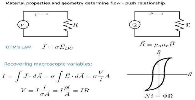
The first is a definition — flux density is simply flux spread over area. The second is a material property, and it is the one that causes trouble, because for iron \(\mu_r\) is not a constant. It depends on \(B\) itself, falling sharply as the material approaches saturation. Chapter 5 makes this precise with the B–H curve. Until then we treat \(\mu_r\) as given and constant, which is honest provided the flux density stays below roughly 1.2 T.
\(H\) is the cause; \(B\) is the effect. You establish \(H\) by choosing a current and a number of turns — it depends only on the coil and the path length, never on what the core is made of. The resulting \(B\) depends entirely on the material, through \(\mu\).
A concrete test of understanding: take a coil establishing \(H = 1000\) AT/m and slide an iron core into it. Does \(H\) change? No — the current and geometry are unchanged. Does \(B\) change? Enormously — from 1.26 mT in air to perhaps 1.26 T in iron of \(\mu_r = 1000\). This is precisely why cores are made of iron.
MMF and Ampère's Circuital Law
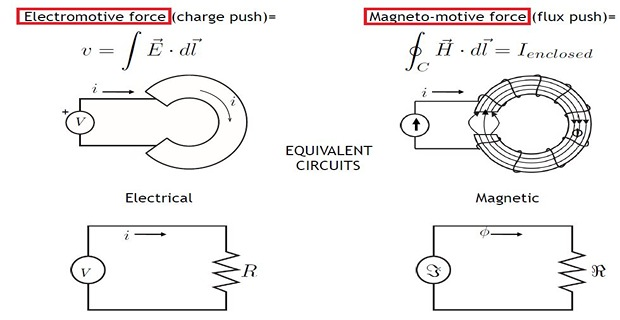
What drives flux around a magnetic path is the magnetomotive force, and where it comes from is Ampère's circuital law. In its general form the law states that the line integral of \(H\) around any closed path equals the total current enclosed by that path:
Now specialise it to a core. If a coil of \(N\) turns carries a current \(I\), the closed path around the core threads that coil \(N\) times, so the enclosed current is \(NI\). If in addition \(H\) is uniform along a path of mean length \(l\) and everywhere parallel to it, the integral is just \(Hl\). Hence
The mmf depends on the product of turns and current, not on either separately. One hundred turns carrying 2 A and two hundred turns carrying 1 A produce identical flux in identical cores. This is the fact that makes transformer design possible, and it is worth pausing on: the coil is a way of multiplying a modest current into a large magnetic drive.
The direction of the flux follows from the right-hand grip rule: curl the fingers of the right hand in the direction the current circulates around the core, and the thumb points along the flux. Reversing the current, or reversing the winding sense, reverses the flux — a fact that becomes important in Chapter 3 when two coils drive the same core, and again in Chapter 52 when three-phase transformer windings must be connected with consistent polarity.
The Magnetic Circuit
A magnetic circuit is the closed path followed by magnetic flux. It is usually built from materials of high permeability — iron, soft steel, silicon steel, ferrite — precisely so that the flux is confined to the intended route rather than wandering through the surrounding air.
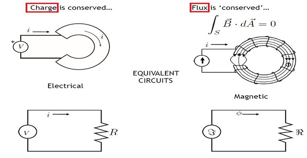
Flux, like current in a wire, leaves a point and returns to the same point after completing its path. There are no magnetic monopoles, so flux lines never begin or end anywhere; they always close on themselves. That is the physical content of \(\nabla \cdot \mathbf{B} = 0\), and it is what licenses the word circuit.
The derivation. Start from the two definitions and Ampère's law, and simply eliminate \(H\) and \(B\):
Substituting this into \(Hl = NI\):
The bracketed quantity in the denominator depends only on the geometry and the material — never on the current. It deserves a name, and it has one: the reluctance \(S\). With that definition the result takes its final form.
Compare with \(I = V/R\) and \(R = \rho l / A\). The correspondence is not a loose resemblance but an exact structural identity, and it means every series–parallel technique from circuit theory applies unchanged. Flux increases if the mmf rises or the reluctance falls, and vice versa.
Two immediate consequences are worth stating explicitly, because students routinely get them backwards:
\(\Phi \propto N\) and \(\Phi \propto I\). Doubling either doubles the flux — provided the iron has not saturated.
\(\Phi \propto 1/S\). A lower reluctance gives a higher flux. Reluctance is opposition, exactly as resistance is.
Problem. A toroidal ring of mean diameter 20 cm and cross-sectional area 5 cm² is wound with 500 turns and carries 2 A. The relative permeability of the core is 800. Find (a) the mmf, (b) the field intensity, (c) the flux density, (d) the flux, and (e) the reluctance. Verify the answer with Hopkinson's law.
(a) MMF.
(b) Field intensity. The mean path length is the circumference at the mean diameter:
(c) Flux density.
(d) Flux.
(e) Reluctance.
Check by Hopkinson's law.
Comment — and a warning. The answer is arithmetically correct but physically suspect: 1.6 T is at or beyond the saturation knee of ordinary silicon steel. At that density the true \(\mu_r\) would be far below 800, so the real flux would be appreciably less than 0.8 mWb. Whenever a calculation of this kind returns a flux density above about 1.5 T, treat the constant-\(\mu_r\) assumption as broken and go to the B–H curve instead (Chapter 5).
Reluctance and Permeance
Reluctance is the opposition a magnetic path offers to the establishment of flux. Its defining expression,
tells you everything about how to reduce it: shorten the path, widen the cross-section, or choose a material of higher permeability. All three appear as design levers in later chapters — the short flux path of a modern induction-motor stator, the generous yoke area of a transformer, and the grain-oriented steel used for both.
The reciprocal quantity is the permeance:
Permeance is to reluctance as conductance is to resistance, and it is used for the same reason: parallel paths add in permeance, which is arithmetically far more comfortable than combining reluctances reciprocally. Chapter 3 leans on this heavily.
Resistance in an ordinary conductor is a genuine constant: double the voltage and you double the current. Reluctance is not, because \(\mu_r\) for iron varies strongly — by a factor of ten or more — with the flux density in the material.
This means a magnetic circuit is a non-linear circuit. Doubling the current does not in general double the flux; past the saturation knee it barely increases it at all. Every constant-\(\mu_r\) calculation in this chapter is therefore an approximation valid over a limited range, and the honest method for a real core is graphical, using the measured B–H curve. Hold that reservation in mind; Chapter 5 removes it.
Problem. A steel ring has a mean circumference of 60 cm and a uniform cross-section of 8 cm². It carries a coil of 400 turns, and the relative permeability of the steel is 1200. What current is needed to establish a flux of 1.0 mWb in the ring?
Solution — the direct route. Work forwards through the chain \(\Phi \to B \to H \to \mathcal{F} \to I\):
Check by the reluctance route. Computing \(S\) first and applying Hopkinson's law must give the same answer:
Both routes are always available. The \(B \to H\) route is preferable when the material is described by a B–H curve rather than a single \(\mu_r\), because \(H\) can then simply be read off the graph. The reluctance route is preferable when several sections must be combined, which is the situation in Chapter 3.
The Magnetic–Electric Analogy
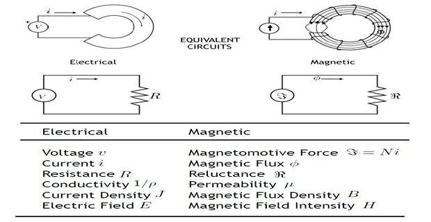
The parallel between Hopkinson's law and Ohm's law runs deeper than the two equations. Term by term, the whole apparatus of DC circuit analysis has a magnetic counterpart, and setting them side by side is the fastest way to become fluent in magnetic circuits.
| Electric circuit | Magnetic circuit | Comment |
|---|---|---|
| EMF, \(V\) (volts) | MMF, \(\mathcal{F} = NI\) (AT) | The driving quantity |
| Current, \(I\) (A) | Flux, \(\Phi\) (Wb) | The response |
| Resistance, \(R = \dfrac{\rho l}{A}\) | Reluctance, \(S = \dfrac{l}{\mu A}\) | The opposition |
| Conductance, \(G = 1/R\) | Permeance, \(P = 1/S\) | Reciprocal opposition |
| Conductivity, \(\sigma\) | Permeability, \(\mu\) | Material property |
| Resistivity, \(\rho\) | Reluctivity, \(1/\mu\) | Specific opposition |
| Current density, \(J = I/A\) | Flux density, \(B = \Phi/A\) | Per unit area |
| Voltage drop, \(IR\) | MMF drop, \(\Phi S = Hl\) | Consumed per section |
| \(I = V/R\) | \(\Phi = \mathcal{F}/S\) | Ohm's and Hopkinson's laws |
| KVL: \(\sum V = \sum IR\) | \(\sum \mathcal{F} = \sum Hl\) | Around any closed loop |
| KCL: \(\sum I = 0\) at a node | \(\sum \Phi = 0\) at a junction | From \(\nabla\cdot\mathbf{B} = 0\) |
| Series: \(R_{eq} = \sum R\) | Series: \(S_{eq} = \sum S\) | Same flux through each |
| Parallel: \(G_{eq} = \sum G\) | Parallel: \(P_{eq} = \sum P\) | Same mmf across each |
The figures below show the correspondence pictorially: in each pair, the magnetic arrangement on one side behaves exactly as the electric arrangement on the other.
Where the Analogy Breaks Down
The analogy is a computational tool, not a statement that flux and current are the same kind of thing. Four differences are important, and examination questions target them relentlessly.
- Flux does not flow. Current is a genuine transport of charge — electrons physically move. Flux is set up, not transported: the molecular dipoles of the material align, and nothing travels around the loop. The word "flow" is a convenient fiction borrowed from the analogy.
- No energy is continuously dissipated. Maintaining a current through a resistance costs \(I^2R\) watts forever. Maintaining a steady flux through a reluctance costs nothing at all — energy is spent only while the flux is being established, and it is stored, not dissipated. (A real coil does dissipate \(I^2R\) in its own winding resistance, but that is the copper's doing, not the magnetic circuit's.) This is why a permanent magnet holds its field indefinitely with no supply.
- There is no magnetic insulator. Electric circuits have excellent insulators — glass, rubber, air — with conductivities a factor of \(10^{20}\) below copper. The best magnetic contrast available is iron against air, a ratio of only a few thousand. Flux will therefore always take some path through the surrounding air, giving rise to leakage flux, which has no electrical counterpart worth speaking of.
- Reluctance is not constant. Resistance is essentially independent of current; reluctance varies with \(B\) because \(\mu_r\) does. A magnetic circuit is intrinsically non-linear, and superposition — the workhorse of linear circuit theory — cannot be applied to a saturating core.
| Aspect | Electric circuit | Magnetic circuit |
|---|---|---|
| Nature of the response | Charge physically flows | Flux is set up; nothing moves |
| Steady-state energy | Continuously dissipated as \(I^2R\) | None — energy is stored, not consumed |
| Insulation | Excellent insulators exist | None; leakage is unavoidable |
| Linearity | \(R\) essentially constant | \(S\) varies with \(B\) — non-linear |
| Temperature effect | \(R\) rises with temperature | \(\mu_r\) falls near the Curie point |
| Analysis method | Algebraic, superposition valid | Often graphical or iterative |
Magnetic Circuits with an Air Gap
Every rotating machine has an air gap — the rotor must be free to turn — and so the composite iron-plus-gap circuit is the single most important configuration in this book. The analysis is a straightforward series combination, but the numerical result is startling the first time you see it.
The iron and the gap carry the same flux, so their reluctances add:
Note the absence of \(\mu_r\) in the second term: for air, \(\mu_r = 1\). Equivalently, in terms of mmf drops,
The length ratio may be tiny, but it is multiplied by \(\mu_r\) — a number in the thousands. A 2 mm gap in a 600 mm iron path of \(\mu_r = 1200\) gives a ratio of \((2/598)(1200) \approx 4\): the air gap has four times the reluctance of the entire iron circuit, despite occupying a third of one percent of the path. This is why machine designers fight for every tenth of a millimetre of clearance.
Problem. The steel ring of Worked Example 2.2 (mean circumference 60 cm, area 8 cm², \(\mu_r = 1200\), 400 turns) has a 2 mm radial slot cut across it. What current is now needed to maintain the same flux of 1.0 mWb? Neglect fringing and leakage.
Solution. The iron path is shortened by the gap:
Iron reluctance.
Gap reluctance. Here \(\mu_r = 1\):
Required mmf and current.
Comment. Compare with 1.243 A for the unbroken ring — a five-fold increase in current to maintain the same flux, caused by removing 2 mm of steel out of 600 mm. The mmf now divides as
Four-fifths of the coil's entire effort is spent pushing flux across two millimetres of air. In a real machine this is not a defect but the price of rotation — and, as Chapter 1 showed, it is also exactly where the useful energy is stored.
Leakage Flux and Fringing
Two effects spoil the tidy picture of Section 2-4, and both follow from the absence of a magnetic insulator. They are distinct, and confusing them is common.
Flux that never reaches the gap at all, closing instead through the air surrounding the core limbs. It is set up by the coil but does no useful work.
The leakage coefficient is typically 1.15 to 1.25 for machines, and much closer to 1.0 for a well-designed transformer. It is always greater than one.
Flux that does cross the gap but bulges outward at the edges, so the effective gap area exceeds the core area. This reduces gap reluctance.
for a rectangular core of face dimensions \(a \times b\). The correction grows with gap length, and is negligible only for very short gaps.
A rough but widely used rule for the fringing correction is to add one gap length to each transverse dimension of the core face — the expression given above. It is empirical, it assumes the gap is short compared with the face dimensions, and it should be regarded as a first-order correction rather than an exact result. For gaps longer than about a tenth of the smaller face dimension, only a field solution will do.
Problem. The core of Worked Example 2.3 has a rectangular cross-section of 20 mm × 40 mm (giving the 8 cm² used earlier) and a 2 mm gap. Recompute the gap reluctance allowing for fringing, and find the corrected current.
Effective gap area. Add one gap length to each transverse dimension:
That is 9.24 cm² against the core's 8 cm² — an increase of 15.5 %.
Corrected gap reluctance.
a reduction of 13.4 % from the uncorrected \(1.9894\times10^{6}\).
Comment. Ignoring fringing overestimated the required current by about 12 % (6.21 A against 5.55 A). Note the direction of the error: neglecting fringing is a conservative mistake — it predicts more current than is actually needed. Neglecting leakage, by contrast, errs the other way and is genuinely dangerous, because it predicts more useful flux than the machine will actually produce.
Applications
The first step in sizing any machine is a magnetic-circuit calculation: choose a working flux density below the saturation knee, compute the core area needed for the required flux, then find the mmf and hence the ampere-turns the winding must supply. Everything else — conductor size, slot dimensions, frame size — follows from that.
A relay is a magnetic circuit with a variable gap. When the armature is open the reluctance is high and the flux is small; as it closes the reluctance collapses and the force rises sharply. This is why relays snap shut rather than closing gently, and why the holding current is far below the pull-in current.
Since flux prefers a low-reluctance path, surrounding a sensitive instrument with a high-permeability shell (mu-metal) diverts stray flux around it rather than through it. The shield does not block the field — there being no magnetic insulator — it merely offers a more attractive route.
If reluctance varies with rotor position, the rotor experiences a torque driving it towards the minimum-reluctance position. That is the whole operating principle of the switched reluctance motor of Chapter 91, and of variable-reluctance position sensors.
A permanent magnet plus a steel pole assembly forms a magnetic circuit whose air gap holds a voice coil. The design goal is a high, uniform \(B\) in a narrow gap — precisely a reluctance-minimisation problem.
Since \(L = N^2/S\), a designer sets inductance by choosing turns and reluctance. A deliberate air gap is often introduced to raise reluctance — lowering \(L\) but allowing far more current before saturation, which is why power inductors are gapped.
Summary and Key Formulas
A magnetic circuit is the closed path taken by flux. Treating it as a circuit is legitimate because iron confines flux much as copper confines current.
Ampère's circuital law applied to a uniform path gives \(Hl = NI\), defining the mmf as the product \(NI\) — turns and current matter only through their product.
Eliminating \(H\) and \(B\) yields Hopkinson's law, \(\Phi = \mathcal{F}/S\), structurally identical to Ohm's law.
Reluctance \(S = l/\mu A\) is reduced by shortening the path, widening it, or raising the permeability. Its reciprocal, permeance, adds for parallel paths and equals \(L/N^2\).
The analogy transfers series and parallel combination, divider rules and both Kirchhoff laws to magnetic circuits.
It fails in four respects: flux does not flow, no steady-state energy is dissipated, no magnetic insulator exists, and reluctance is not constant.
An air gap of a fraction of a percent of the path length can dominate the total reluctance, because the length ratio is multiplied by \(\mu_r\). Expect the gap to consume most of the mmf.
Leakage reduces useful flux and is handled by a coefficient greater than one; fringing lowers gap reluctance and is handled by enlarging the effective gap area. They are opposite effects.
| Quantity | Formula | Notes |
|---|---|---|
| Flux density | \(B = \dfrac{\Phi}{A}\) | tesla; a definition |
| Material relation | \(B = \mu_0\mu_r H\) | \(\mu_r\) is not constant for iron |
| Ampère's law | \(\oint \mathbf{H}\cdot\mathrm{d}\mathbf{l} = \sum i\) | general form |
| MMF | \(\mathcal{F} = NI = Hl\) | ampere-turns |
| Hopkinson's law | \(\Phi = \dfrac{\mathcal{F}}{S}\) | the magnetic Ohm's law |
| Reluctance | \(S = \dfrac{l}{\mu_0\mu_r A}\) | AT/Wb |
| Permeance | \(P = \dfrac{1}{S}\) | adds for parallel paths |
| Series reluctance | \(S_{eq} = S_1 + S_2 + \cdots\) | same flux in each section |
| Air-gap reluctance | \(S_g = \dfrac{l_g}{\mu_0 A_g}\) | no \(\mu_r\) — air |
| MMF drop per section | \(\mathcal{F}_k = \Phi S_k = H_k l_k\) | sums to the total mmf |
| Fringing correction | \(A_g \approx (a+l_g)(b+l_g)\) | empirical; short gaps only |
| Leakage coefficient | \(\lambda_{\text{lk}} = \dfrac{\Phi_{\text{total}}}{\Phi_{\text{useful}}}\) | always \(> 1\); 1.15–1.25 typical |
| Flux linkage | \(\lambda = N\Phi\) | weber-turns |
| Inductance | \(L = \dfrac{N^{2}}{S} = N^{2}P\) | developed in Chapter 13 |
Common Mistakes
Confusing \(B\) with \(H\). \(H\) is set by the coil and geometry alone; \(B\) depends on the material. Inserting iron changes \(B\) enormously and leaves \(H\) untouched.
Including \(\mu_r\) in the air-gap reluctance. For air \(\mu_r = 1\). Carrying the iron's \(\mu_r\) into the gap term understates the gap reluctance by a factor of thousands, and is the single most damaging arithmetic slip in this chapter.
Forgetting to subtract the gap from the iron path length. If the mean path is 60 cm and a 2 mm gap is cut, the iron is 59.8 cm, not 60 cm. The error is small here but grows for large gaps.
Mixing units. Areas in cm² and lengths in cm, dropped into a formula expecting SI. Convert everything to metres and square metres before substituting: 1 cm² = \(10^{-4}\) m², 1 mm = \(10^{-3}\) m.
Treating mmf as a force. Despite its name, magnetomotive force is not a force and is not measured in newtons. Nor is electromotive force. Both names are historical accidents.
Adding reluctances in parallel as if they were in series. Parallel paths share the mmf and divide the flux; add their permeances, or combine reluctances reciprocally.
Assuming reluctance is constant. It is not, and any answer returning \(B\) above about 1.5 T should be treated as suspect until checked against the B–H curve.
Confusing leakage with fringing. Leakage never crosses the gap and reduces useful flux; fringing does cross the gap and reduces its reluctance. Their effects on the answer point in opposite directions.
Believing a magnetic circuit dissipates power in the reluctance. It does not. The \(I^2R\) heat comes from the copper of the coil, not from the magnetic path. A steady flux is free to maintain.
Applying superposition to a saturated core. Superposition requires linearity. Two coils on a saturating core do not produce the sum of the fluxes each would produce alone.
Chapter Review
Work these before opening the answers. Convert all quantities to SI units first — most errors in this chapter are unit errors, not conceptual ones.
P2.1 A toroid of mean length 0.5 m and cross-section 4 cm² carries 600 turns at 1.5 A. The core has \(\mu_r = 500\). Find the mmf, \(H\), \(B\), \(\Phi\) and \(S\).
Show answer
\[\mathcal{F} = (600)(1.5) = 900~\mathrm{AT}, \qquad H = \frac{900}{0.5} = 1800~\mathrm{AT/m}\]\[\mu = (4\pi\times10^{-7})(500) = 6.283\times10^{-4}, \qquad B = (6.283\times10^{-4})(1800) = 1.131~\mathrm{T}\]\[\Phi = (1.131)(4\times10^{-4}) = 4.524\times10^{-4}~\mathrm{Wb} = 0.452~\mathrm{mWb}\]Check: \(\Phi = 900/1.989\times10^{6} = 4.52\times10^{-4}\) Wb \(\checkmark\)\[S = \frac{0.5}{(6.283\times10^{-4})(4\times10^{-4})} = 1.989\times10^{6}~\mathrm{AT/Wb}\]P2.2 Find the reluctance of an air gap 1 mm long and 10 cm² in area.
Show answer
Note there is no \(\mu_r\) term. For comparison, a metre of iron of the same area with \(\mu_r = 2000\) would have \(S = 3.98\times10^{5}\) AT/Wb — half as much, from a thousand times the length.\[S_g = \frac{l_g}{\mu_0 A_g} = \frac{1\times10^{-3}}{(4\pi\times10^{-7})(1\times10^{-3})} = \frac{10^{-3}}{1.2566\times10^{-9}} = 7.958\times10^{5}~\mathrm{AT/Wb}\]P2.3 A sample of steel is found to have \(B = 1.1\) T when \(H = 550\) AT/m. Find its permeability and relative permeability.
Show answer
\[\mu = \frac{B}{H} = \frac{1.1}{550} = 2.00\times10^{-3}~\mathrm{H/m}\]\[\mu_r = \frac{\mu}{\mu_0} = \frac{2.00\times10^{-3}}{4\pi\times10^{-7}} = 1592\]P2.4 A magnetic circuit of reluctance \(3\times10^{6}\) AT/Wb is driven by 1500 AT. Find the flux. If the coil has 750 turns, what current flows?
Show answer
\[\Phi = \frac{1500}{3\times10^{6}} = 5.00\times10^{-4}~\mathrm{Wb} = 0.500~\mathrm{mWb}\]\[I = \frac{1500}{750} = 2.00~\mathrm{A}\]P2.5 A coil of 200 turns produces a flux of 0.6 mWb. Without changing the core, the turns are increased to 500 and the current halved. What is the new flux, assuming no saturation? What if the core is saturated?
Show answer
The mmf changes in the ratio \((500 \times 0.5)/(200 \times 1) = 1.25\), soIf saturated, the proportionality fails entirely: past the knee, a 25 % rise in mmf might produce only a few percent more flux. The linear answer is then an upper bound, and only the B–H curve gives the truth.\[\Phi' = (0.6)(1.25) = 0.750~\mathrm{mWb}\]P2.6 An iron ring of mean iron path 40 cm and cross-section 5 cm² has a 1 mm air gap and carries 800 turns. Take \(\mu_r = 1500\) and neglect fringing and leakage. Find the current needed for a flux of 0.6 mWb, and the percentage of mmf absorbed by the gap.
Show answer
Iron: \(H_i = B/(\mu_0\mu_r) = 1.20/(1.885\times10^{-3}) = 636.6\) AT/m, so\[B = \frac{0.6\times10^{-3}}{5\times10^{-4}} = 1.20~\mathrm{T}\]Gap: \(H_g = B/\mu_0 = 1.20/(1.2566\times10^{-6}) = 9.549\times10^{5}\) AT/m, so\[\mathcal{F}_i = (636.6)(0.40) = 254.6~\mathrm{AT}\]\[\mathcal{F}_g = (9.549\times10^{5})(0.001) = 954.9~\mathrm{AT}\]The gap takes \(954.9/1209.5 = 78.9\,\%\) of the mmf.\[\mathcal{F} = 254.6 + 954.9 = 1209.5~\mathrm{AT} \quad\Longrightarrow\quad I = \frac{1209.5}{800} = 1.51~\mathrm{A}\]P2.7 Two magnetic paths of reluctance \(4\times10^{5}\) and \(6\times10^{5}\) AT/Wb are in parallel across a common mmf. Find the equivalent reluctance, and the fraction of the total flux in each.
Show answer
Work in permeances, which add in parallel:\[P_{eq} = \frac{1}{4\times10^{5}} + \frac{1}{6\times10^{5}} = 2.5\times10^{-6} + 1.667\times10^{-6} = 4.167\times10^{-6}\]Flux divides inversely as reluctance: \(\Phi_1/\Phi = 2.5/4.167 = 60\,\%\) and \(\Phi_2/\Phi = 40\,\%\). The lower-reluctance path carries more flux — exactly as the lower resistance carries more current.\[S_{eq} = \frac{1}{4.167\times10^{-6}} = 2.40\times10^{5}~\mathrm{AT/Wb}\]P2.8 A machine's coil sets up a total flux of 1.25 mWb, of which 1.05 mWb crosses the air gap. Find the leakage coefficient and the leakage flux.
Show answer
\[\lambda_{\text{lk}} = \frac{1.25}{1.05} = 1.190\]A coefficient of 1.19 is typical of a rotating machine. A transformer would be far closer to 1.0.\[\Phi_{\text{leak}} = 1.25 - 1.05 = 0.20~\mathrm{mWb} \quad (16\,\% \text{ of the total})\]P2.9 A core operating at \(\mu_r = 2000\) is driven harder until \(\mu_r\) falls to 400. By what factor does the iron reluctance change, and what does this do to the flux for a fixed mmf?
Show answer
Since \(S \propto 1/\mu_r\), the reluctance rises by a factor of \(2000/400 = 5\). For a fixed mmf the flux therefore falls to one-fifth of what the linear model would predict.This is saturation in one line: past the knee, extra current buys very little extra flux, and the constant-\(\mu_r\) model becomes badly optimistic.\[S' = 5S \quad\Longrightarrow\quad \Phi' = \frac{\mathcal{F}}{5S} = \frac{\Phi_{\text{linear}}}{5}\]P2.10 A rectangular core face measures 25 mm × 50 mm with a 3 mm gap. Find the gap reluctance with and without the fringing correction, and the percentage error incurred by ignoring it.
Show answer
Without fringing, \(A_g = (0.025)(0.050) = 1.25\times10^{-3}\) m²:With fringing, \(A_g = (0.028)(0.053) = 1.484\times10^{-3}\) m²:\[S_g = \frac{0.003}{(4\pi\times10^{-7})(1.25\times10^{-3})} = \frac{0.003}{1.5708\times10^{-9}} = 1.910\times10^{6}~\mathrm{AT/Wb}\]Ignoring fringing overestimates the gap reluctance by \((1.910-1.609)/1.609 = 18.7\,\%\). The error is larger than in Example 2.4 because the gap is longer relative to the face dimensions — which is also the warning that the empirical correction is nearing the limit of its validity.\[S_g' = \frac{0.003}{(4\pi\times10^{-7})(1.484\times10^{-3})} = \frac{0.003}{1.8650\times10^{-9}} = 1.609\times10^{6}~\mathrm{AT/Wb}\]
MCQ 1. The unit of magnetomotive force is:
(a) weber (b) tesla (c) ampere-turn (d) ampere-turn per metreShow answer
(c) ampere-turn. Ampere-turn per metre is the unit of \(H\); weber is flux and tesla is flux density.MCQ 2. Reluctance is given by:
(a) \(\mu A / l\) (b) \(l / \mu A\) (c) \(l A / \mu\) (d) \(\mu l / A\)Show answer
(b) \(l/\mu A\). Compare \(R = \rho l/A\), with \(1/\mu\) playing the role of \(\rho\).MCQ 3. In the magnetic–electric analogy, flux corresponds to:
(a) voltage (b) current (c) resistance (d) powerShow answer
(b) current. MMF corresponds to voltage and reluctance to resistance.MCQ 4. Inserting an iron core into a current-carrying coil:
(a) increases \(H\) only (b) increases \(B\) only (c) increases both (d) changes neitherShow answer
(b) increases \(B\) only. \(H = NI/l\) is fixed by the coil and geometry; only the material-dependent \(B = \mu H\) responds.MCQ 5. A 1 mm air gap in a 50 cm iron path of \(\mu_r = 2000\) has a reluctance, relative to the iron, of about:
(a) one-quarter (b) equal (c) four times (d) forty timesShow answer
(c) four times. \(S_g/S_i = (l_g/l_i)\mu_r = (1/499)(2000) \approx 4.0\).MCQ 6. Which of these has no counterpart in an electric circuit?
(a) series combination (b) Kirchhoff's current law (c) leakage flux (d) a divider ruleShow answer
(c) leakage flux. Good electrical insulators exist, so current does not leak appreciably. There is no magnetic insulator, so flux always does.MCQ 7. Maintaining a steady flux in a magnetic circuit requires:
(a) continuous power in the reluctance (b) no power in the reluctance (c) power proportional to \(\Phi^2 S\) (d) power proportional to \(\Phi S\)Show answer
(b) no power in the reluctance. Energy is stored while the flux is established, not dissipated thereafter. Any heat comes from the coil's own resistance.MCQ 8. Fringing at an air gap:
(a) increases gap reluctance (b) decreases gap reluctance (c) has no effect (d) reverses the fluxShow answer
(b) decreases it, because the flux spreads over an effective area larger than the core cross-section.MCQ 9. The leakage coefficient of a machine is always:
(a) less than 1 (b) equal to 1 (c) greater than 1 (d) negativeShow answer
(c) greater than 1, since it is total flux divided by useful flux and some flux always leaks.MCQ 10. Permeance is measured in:
(a) AT/Wb (b) henries (c) teslas (d) webersShow answer
(b) henries. Permeance is Wb/AT, which is dimensionally a henry — and indeed \(L = N^2 P\).
The magnetic–electric analogy is exact at the level of the governing equation but false at the level of physics. Identify the equation-level correspondence and then state, in your own words, what is physically different about flux and current.
A steady current through a resistance dissipates power forever, yet a steady flux through a reluctance dissipates nothing. Given that both obey the same algebraic law, explain where the asymmetry enters.
Why does the absence of a magnetic insulator matter so much more for a rotating machine than for a transformer?
A student proposes eliminating the air gap in a motor to reduce the required mmf. Explain both why the proposal is arithmetically sound and why it is physically absurd.
Superposition is valid in linear electric circuits. Explain precisely which property of iron makes it invalid for a magnetic circuit, and identify the operating region in which it becomes approximately usable again.
Two coils of different turn counts produce the same flux in the same core. What must be true of their currents, and what does this tell you about the design freedom available to a transformer designer?
Neglecting fringing overestimates the required current, while neglecting leakage overestimates the useful flux. Explain why the second error is the more dangerous of the two in practice.
This chapter handled a single flux path. Real cores rarely oblige: a transformer core has a central limb carrying flux that divides between two outer limbs, and a machine has several parallel routes through teeth, yoke and gap. Chapter 3 extends the analogy to series and parallel magnetic circuits, where the two Kirchhoff analogues of Table 2.2 come into their own, and where the composite core of Analogy 4 is solved properly.
Chapter 4 then confronts the air gap in earnest — fringing, leakage and the practical corrections engineers actually apply — and Chapter 5 finally discharges the debt this chapter has been quietly accumulating, by replacing the fictional constant \(\mu_r\) with the measured B–H curve. From there, Chapters 6 and 7 show what all this flux-shuffling costs in heat.