Alternator Voltage Control: Methods & Techniques | Electrical Machines

Demonstrative Video

SECTION 01

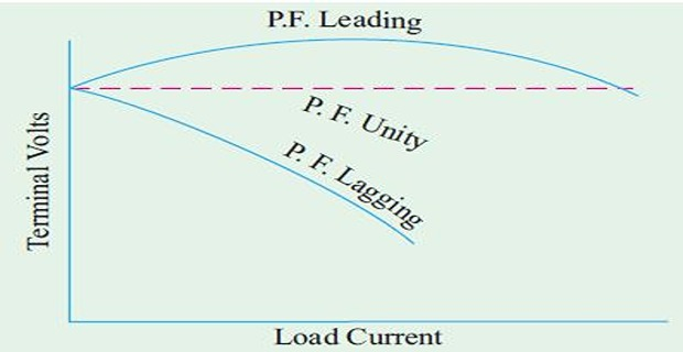
Voltage Regulation

\[\boxed{\% \mbox{Voltage Reg.} = \dfrac{E_0-V}{V} \times 100}\]
remaining the same) divided by the rated terminal voltage and It is defined as the rise in voltage when full-load is removed (

The magnitude of the change in \(V\) depends not only on the load but also on the load power factor

Direct Method- for small machines

- Direct Method - for small machines
- Indirect Method - for large machines

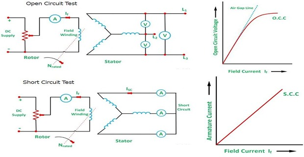
Alternator is driven at \(N_s\) and \(V\) is adjusted to rated value
Vary the load until watt-meter and ammeter indicates the rated values at desired p.f.
Throw the entire load off keeping the \(N\) and \(I_f\) constant
\[\% V.R. = \dfrac{E_0-V}{V} \times 100\]
is read Open-circuit or no-load voltage
Large machines the cost to find the regulation by direct loading becomes prohibitive.

All these methods require-

All these methods require-
1. Armature resistance \(R_a\)
  - obtained by direct measurement (Voltmeter-ammeter or Wheatstone bridge)
2. Open-circuit/No-load Characteristic
3. Short-circuit characteristic (but ZPF lagging for Potier)

Test Regulation

- Not accurate;foundthan its value at normal voltage conditions and saturation

\[\begin{aligned} Z_s & = \dfrac{E_1(\mbox{open-circuit})}{I_1(\mbox{short-circuit})} ~~ X_s=\sqrt{Z_s^2-R_a^2}\\ E_{0}&=\sqrt{\left(V\cos\phi+IR_{a}\right)^{2}+\left(V\sin\phi+IX_{s}\right)^{2}} \end{aligned}\]

- Not accurate; \(Z_s\) found \(>\) than its value at normal voltage conditions and saturation.
\(X_a\) has not been treated separately but along with \(X_L\)

Converse of the EMF method:is treated as an additional AR

Converse of the EMF method: \(X_L\) is treated as an additional AR
Field A.T. required for \(V\) on F.L. is the vector sum of
- O.C. test : Field A.T. required for \(V\) (or if \(R_a\) is to be taken into account, then \(V+IR_a\cos \phi\)) on no-load
- S.C. test: Field A.T. to overcome demagnetising effect of AR on F.L. Field A.T. required to produce F.L. current on S.C balance the armature reaction and the impedance drop
  - \(Z_s\) drop neglected, \(R_a\) very small and \(X_s\) also small under S.C. condition
  - P.F. on S.C is almost zero lagging and field A.T. are used entirely to overcome AR which is wholly demagnetising

representsfor

\(OA\) represents \(I_f\) for \(V\)
\(OC\) represents \(I_f\) required to produce F.L current on S.C
\(\overrightarrow{AB} = \overrightarrow{OC}\) drawn at \((90^{\circ})+\phi\) to \(OA\) (p.f. lagging)
Total \(I_f\) is \(OB\) for which the corresponding O.C. voltage is \(E_0\)
: give results less than the actual value

Key Concepts

method based on separation of armature-leakage reactance drop and the armature reaction effects
gives more accurate results
makes use of first two methods
OCC and F.L. ZPF (not SCC)
ZPF curve - \(V\) against \(I_f\) when delivering \(I_{a,F.L}\) at zero p.f.
Note \(\boxed{E_0 = \left[V + I_a(R_a+jX_L)\right]+ \mbox{armature-reaction drop}}\) (assuming lagging p.f.)

Point- wattmeter =

Point \(B\) - wattmeter = \(0\)
Point \(A\) - SC test with F.L \(I_a\)
\(OA\) represents \(I_f\) = and opposite to demagnetising armature reaction and for balancing \(X_L\) drop at F.L.
From \(B\), draw \(BH\) = and \(\parallel\) \(OA\)
From \(H\), \(HD\) drawn \(\parallel\) initial straight part of NL curve, i.e. \(\parallel\) \(OC\), which is tangential to the NL curve

We get point \(D\) on NL curve, which corresponds to point \(B\) on F.L. ZPF curve
Triangle \(BHD\) is Potier triangle

Potier1Potier

Potier1

Potier

Draw \(DE\) \(\perp\) \(BH\)
\(DE\) = \(IX_L\)
\(BE\), \(I_f\) to overcome demagnetising effect of AR at FL
\(EH\) for balancing \(X_L\) drop \(DE\)
\(E=DF=V+jIX_L\) (neglecting \(R_a\)); \(I_f = OF\)
\(NA = BE\) represents \(I_f\) needed to overcome AR
\(\overrightarrow{NA}+\overrightarrow{OF}\), \(I_f\) for \(E_0\), read from NL curve (\(NA=FG\))