By the end of this chapter you should be able to:
Classify the losses of a DC machine and give typical magnitudes.
Distinguish constant from variable losses and justify each assignment.
Draw the power-flow diagram for a generator and for a motor.
Work through the power stages and compute efficiency at each.
Derive the condition for maximum efficiency.
Find the load current at which maximum efficiency occurs.
Explain the shape of the efficiency curve and why it is flat near the top.
Use the loss breakdown to say where to look for an improvement.
Classification of Losses
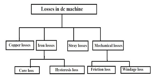
| Loss | Origin | Typical magnitude | Varies with |
|---|---|---|---|
| Armature copper | Current in the armature winding | 3–6 % | \(I_a^{2}\) |
| Field copper | Current in shunt and series fields | 1–5 % | constant (shunt), \(I^{2}\) (series) |
| Iron | Alternating magnetisation of the armature core | — | speed and flux |
| Mechanical | Friction and windage | 3–15 % (with iron) | speed |
| Stray | Armature reaction, commutation currents | 1 % of full-load output | load, approximately |
Copper Losses
These occur generally due to current in the various windings.
The armature copper loss is typically 3–6 % of rated output and the field losses 1–5 %.
The loss at the brush contact resistance is conventionally included in the armature copper loss, though it does not follow an \(I^{2}R\) law.
Chapter 22 showed why: the carbon-copper contact has a roughly constant voltage drop of about 1 V per brush, so the loss is
which is proportional to \(I_a\), not to \(I_a^{2}\). It is grouped with the armature loss because it varies with load, which is what matters for the classification of Section 33-5, not because the physics is the same.
Iron Losses
These are the losses within the armature due to its rotation within the magnetic field of the poles.
where \(V\) is the volume of iron and \(f\) the frequency of magnetisation.
Chapter 27 supplied the frequency: the armature iron is magnetised alternately north and south at
so both components rise with speed — hysteresis in proportion, eddy current as the square. Iron loss is therefore a function of speed and flux, and not of load current at all, which is what puts it among the constant losses of Section 33-5.
The qualification is that "constant" means constant with respect to load. A machine run at a different speed, or with its field weakened, has a different iron loss — which is why the speed-control methods of Chapter 37 change the efficiency as well as the speed.
Mechanical and Stray Losses
Friction: in bearings, at the brushes, and in any seals.
Windage: air friction on the rotating armature and any cooling fan.
These depend on the speed of the machine and not on the load. Together with the iron losses they amount to 3–15 %.
Miscellaneous losses occurring because of:
Distortion of flux due to armature reaction.
Short-circuit currents in the coil undergoing commutation.
These are very difficult to determine, so a reasonable value is assigned — conventionally 1 % of full-load output power.
Constant and Variable Losses
For the efficiency analysis that follows, the losses are regrouped by how they behave as the load changes.
Iron losses
Mechanical losses
Shunt field losses
Copper loss in the armature
Copper loss in the series field
Because the shunt field is connected across the terminals, and the terminal voltage is held roughly constant. From Chapter 26, \(I_{sh} = V/R_{sh}\), so
which does not involve the load current at all. The series field, by contrast, carries the load current, so its loss varies as \(I^{2}\) and belongs firmly with the variable losses.
Power Flow in DC Machines
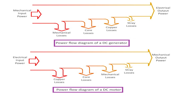
Mechanical power in, electrical power out. The rotational losses are taken off first, since they are incurred before any conversion.
Electrical power in, mechanical power out — the same chain read backwards, with \(E_b\) in place of \(E_g\).
Everything on the electrical side of this product is copper and brush loss; everything on the mechanical side is iron and friction. The iron loss sits on the mechanical side of the ledger even though it is an electromagnetic effect — it is supplied by the shaft, not by the terminals.
Power Stages and Efficiency
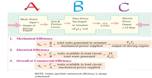
| Efficiency | Definition | Accounts for |
|---|---|---|
| Mechanical | \(\eta_m = \dfrac{E_gI_a}{P_{\text{mech,in}}}\) | iron and friction losses |
| Electrical | \(\eta_e = \dfrac{VI_L}{E_gI_a}\) | copper and brush losses |
| Commercial or overall | \(\eta = \dfrac{VI_L}{P_{\text{mech,in}}} = \eta_m\eta_e\) | everything |
The commercial efficiency is the product of the other two, and it is the only one a purchaser cares about.
Problem. A 20 kW, 250 V shunt generator has \(R_a = 0.10~\Omega\), \(R_{sh} = 125~\Omega\), a brush drop of 1 V per brush, iron and mechanical losses totalling 600 W, and stray losses of 1 % of output. Find every loss and the efficiency at full load.
Currents.
| Loss | Expression | Value | Class |
|---|---|---|---|
| Armature copper | \((82)^{2}(0.10)\) | 672.4 W | variable |
| Brush contact | \((2)(1)(82)\) | 164.0 W | variable |
| Shunt field | \((250)(2)\) | 500.0 W | constant |
| Iron and mechanical | given | 600.0 W | constant |
| Stray | \((0.01)(20\,000)\) | 200.0 W | — |
| Total | 2136.4 W |
Input and efficiency.
Comment. The armature copper loss is 3.36 % of output, comfortably inside the 3–6 % band of Table 33.1, and the field loss 2.5 %. The largest single item is the iron and mechanical loss at 600 W, which no amount of load reduction will diminish — a point Section 33-9 turns into the condition for maximum efficiency.
Note that a designer looking to improve this machine would attack the 600 W first, since it is both the largest item and the one that penalises light-load operation most heavily.
Condition for Maximum Efficiency
For a generator delivering current \(I\) at terminal voltage \(V\):
If \(I_{sh}\) is negligible compared with the load current, then \(I_a \approx I\) and
Dividing numerator and denominator by \(VI\):
Efficiency is maximum when the denominator is minimum, that is when
At that current the total loss is exactly \(2W_c\), evenly divided between the two families.
The result is general. It holds for transformers, for AC machines, and indeed for any device whose losses split into a term independent of load and a term proportional to its square — a fact worth remembering, because it will reappear in Part 3.
Problem. For the generator of Example 33.1, take the constant losses as the shunt field plus the iron and mechanical losses. Find the load current for maximum efficiency, express it as a fraction of full load, and find the efficiency there.
Constant losses.
Current for maximum efficiency.
As a fraction of full load.
Efficiency there. The total loss is \(2W_c = 2200\) W:
Comment. Maximum efficiency occurs at 131 % of rated load — a load the machine is not designed to carry continuously. This machine is therefore never operated at its own best point, and its constant losses are too high relative to its armature resistance.
That is not necessarily a fault. Machines expected to run mostly at part load are deliberately designed with the maximum below full load, so the efficiency is high where the machine actually works. The design target is a matter of the duty cycle, not of the peak value.
Problem. What would have to change for the generator of Example 33.2 to reach maximum efficiency exactly at its rated 80 A?
Setting the condition at full load.
Option 1 — reduce the constant losses.
Achievable by thinner laminations, better bearings, or a higher-resistance shunt field with more turns.
Option 2 — increase the armature resistance.
Comment. Option 2 is arithmetically valid and practically absurd. Deliberately worsening the armature to move the efficiency peak would lower the efficiency at every load, including the new peak — the machine would reach its maximum at 80 A, but that maximum would be worse than the 92.0 % it already achieves there.
The lesson is that the condition \(I^{2}R_a = W_c\) locates the peak but says nothing about its height. Only Option 1 improves the machine, because it reduces a loss rather than redistributing it.
The Efficiency Curve
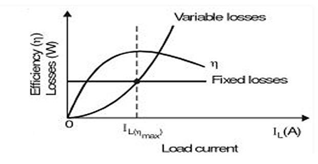
At low load the constant loss \(W_c\) is a large fraction of a small output, so efficiency is poor and rises steeply as the load increases.
Near the maximum the two loss terms are comparable and moving in opposite directions, so their sum changes very little — the curve is flat.
Beyond the maximum the \(I^{2}R_a\) term dominates and efficiency falls slowly.
The flatness at the top is why the exact location of the maximum matters less than one might expect — but the steepness at the bottom is why running a machine at a small fraction of its rating is genuinely wasteful.
Problem. Tabulate the efficiency of the generator of Example 33.2 from a quarter load to 150 % load, using \(W_c = 1100\) W and \(R_a = 0.10~\Omega\) and neglecting brush and stray losses.
| \(I\) (A) | % of full load | Output (W) | Variable loss (W) | Total loss (W) | \(\eta\) |
|---|---|---|---|---|---|
| 20 | 25 | 5000 | 40 | 1140 | 81.43 % |
| 40 | 50 | 10 000 | 160 | 1260 | 88.81 % |
| 60 | 75 | 15 000 | 360 | 1460 | 91.13 % |
| 80 | 100 | 20 000 | 640 | 1740 | 92.00 % |
| 104.9 | 131 | 26 220 | 1100 | 2200 | 92.26 % |
| 120 | 150 | 30 000 | 1440 | 2540 | 92.19 % |
Working for the 40 A row.
Comment. Between full load and the true maximum the efficiency gains only 0.26 percentage points, and it is still 92.19 % at 150 % load. The top of the curve is nearly flat over a two-to-one range of current.
The contrast at the other end is stark: at quarter load the efficiency has fallen to 81.4 %, more than ten points below the peak, because the unchanging 1100 W is now 22 % of the output. This is the arithmetic behind Chapter 32's argument for shutting units down as the station load falls — two machines at 90 % beat four at 45 %.
Problem. A 230 V shunt motor takes 50 A from the supply. Its armature resistance is 0.20 \(\Omega\), shunt field resistance 115 \(\Omega\), brush drop 1 V per brush, and iron plus friction losses 400 W. Find the power at each stage and the efficiency.
Currents.
Note the minus sign — for a motor the line current splits between armature and field.
Stage 1 — electrical input.
Stage 2 — after the field loss.
Stage 3 — after the armature and brush losses.
Check: \(11\,500 - 460 - 460.8 - 96 = 10\,483.2\) W \(\checkmark\)
Stage 4 — shaft output.
Efficiency.
Comment. The converted power \(E_bI_a\) is the pivot of the whole calculation, exactly as \(E_gI_a\) was for the generator. Above it lies the electrical world, below it the mechanical, and the two are joined by the machine constant of Chapter 27.
Note that the field takes 460 W — 4 % of the input — purely to magnetise the machine, producing no output at all. In a permanent-magnet motor that loss is absent, which is one of the reasons Chapter 26 gave for their use in small sizes.
Summary and Key Formulas
Copper losses are \(I_a^{2}R_a\) (3–6 %), \(I_{sh}^{2}R_{sh}\) and \(I_{se}^{2}R_{se}\) (1–5 %). Brush contact loss \(2v_bI_a\) is conventionally grouped with the armature loss.
Iron losses are \(K_hB_{max}^{1.6}fV\) and \(K_eB_{max}^{2}f^{2}V\), with \(f = PN/120\). They depend on speed and flux, not on load.
Mechanical losses — friction and windage — depend on speed. With iron losses they total 3–15 %.
Stray losses arise from armature reaction and commutation, and are assigned a value of 1 % of full-load output.
Constant losses: iron, mechanical and shunt field. Variable losses: armature and series-field copper.
Power flow, generator: mechanical input \(\to\) \(E_gI_a\) \(\to\) \(VI_a\) \(\to\) \(VI_L\). For a motor the same chain runs backwards with \(E_b\).
Efficiency \(\eta = VI/(VI + I^{2}R_a + W_c)\), and \(\eta = \eta_m\eta_e\).
Maximum efficiency occurs when variable loss equals constant loss, at \(I = \sqrt{W_c/R_a}\), where the total loss is \(2W_c\).
The efficiency curve is steep at low load and flat near the maximum, so part-load operation is costly but the exact peak location is not critical.
| Quantity | Formula | Notes |
|---|---|---|
| Armature copper loss | \(I_a^{2}R_a\) | variable |
| Brush loss | \(2v_bI_a\) | varies as \(I_a\), not \(I_a^{2}\) |
| Shunt field loss | \(VI_{sh} = V^{2}/R_{sh}\) | constant |
| Hysteresis loss | \(K_hB_{max}^{1.6}fV\) | \(f = PN/120\) |
| Eddy current loss | \(K_eB_{max}^{2}f^{2}V\) | — |
| Stray loss | 1 % of full-load output | by convention |
| Converted power | \(E_gI_a\) or \(E_bI_a\) | the pivot of the diagram |
| Mechanical efficiency | \(\eta_m = E_gI_a/P_{\text{mech}}\) | generator |
| Electrical efficiency | \(\eta_e = VI_L/E_gI_a\) | generator |
| Overall efficiency | \(\eta = \eta_m\eta_e\) | commercial efficiency |
| Maximum efficiency | \(I = \sqrt{W_c/R_a}\) | variable = constant |
| Loss at maximum | \(2W_c\) | evenly split |
Common Mistakes
Using \(I_L\) in the armature copper loss. It is \(I_a^{2}R_a\), and \(I_a = I_L + I_{sh}\) for a generator, \(I_L - I_{sh}\) for a motor.
Treating the brush loss as \(I_a^{2}R_b\). The contact drop is roughly constant, so the loss is \(2v_bI_a\).
Putting the shunt field loss among the variable losses. It is \(V^{2}/R_{sh}\) and does not involve the load.
Putting the series field loss among the constant losses. It carries the load current and varies as \(I^{2}\).
Calling iron loss constant in an absolute sense. It is constant with respect to load, but changes with speed and flux.
Taking the rotational losses off the wrong side. They belong on the mechanical side of \(E_gI_a\), not the electrical side.
Using \(\eta = \text{output}/(\text{output} + \text{losses})\) for a motor with the electrical output. A motor's output is mechanical; its input is electrical.
Assuming maximum efficiency occurs at full load. It occurs where \(I^{2}R_a = W_c\), which may be well above or below rated load.
Thinking the condition tells you the value of the maximum. It locates the peak only; reducing a loss is what raises it.
Forgetting that efficiency collapses at light load. The constant loss is unchanged while the output shrinks.
Chapter Review
Find \(I_a\) first — with the correct sign for a generator or a motor — then list the losses by class.
P33.1 A 10 kW, 200 V shunt generator has \(R_a = 0.15~\Omega\), \(R_{sh} = 100~\Omega\) and iron plus mechanical losses of 400 W. Find the full-load efficiency, neglecting brush and stray losses.
Show answer
\[I_L = 50~\mathrm{A}, \quad I_{sh} = 2~\mathrm{A}, \quad I_a = 52~\mathrm{A}\]\[I_a^{2}R_a = (2704)(0.15) = 405.6~\mathrm{W}, \quad VI_{sh} = 400~\mathrm{W}\]\[\text{total loss} = 405.6 + 400 + 400 = 1205.6~\mathrm{W}\]\[\eta = \frac{10\,000}{11\,205.6} = 89.24\,\%\]P33.2 For P33.1, find the load current at which efficiency is maximum and the value there.
Show answer
\[W_c = 400 + 400 = 800~\mathrm{W}, \qquad I = \sqrt{\frac{800}{0.15}} = 73.03~\mathrm{A}\]\[P_{\text{out}} = (200)(73.03) = 14\,606~\mathrm{W}, \qquad \text{loss} = 1600~\mathrm{W}\]This is 146 % of full load, so again the machine never reaches its own peak.\[\eta_{\max} = \frac{14\,606}{16\,206} = 90.13\,\%\]P33.3 A machine has constant losses of 900 W and an armature resistance of 0.05 \(\Omega\). At what current is efficiency maximum, and what is the total loss there?
Show answer
\[I = \sqrt{\frac{900}{0.05}} = \sqrt{18\,000} = 134.2~\mathrm{A}\]\[\text{total loss} = 2W_c = 1800~\mathrm{W}\]P33.4 A 240 V shunt motor takes 40 A. With \(R_a = 0.25~\Omega\), \(R_{sh} = 120~\Omega\) and rotational losses of 350 W, find the output and efficiency. Neglect brush drop.
Show answer
\[I_{sh} = 2~\mathrm{A}, \qquad I_a = 40 - 2 = 38~\mathrm{A}\]\[P_{\text{in}} = (240)(40) = 9600~\mathrm{W}\]\[E_b = 240 - (38)(0.25) = 230.5~\mathrm{V}, \qquad P_{\text{conv}} = (230.5)(38) = 8759~\mathrm{W}\]\[P_{\text{out}} = 8759 - 350 = 8409~\mathrm{W}, \qquad \eta = \frac{8409}{9600} = 87.59\,\%\]P33.5 A machine with \(W_c = 1000\) W and \(R_a = 0.08~\Omega\) runs at 60 A and at 200 V. Find its efficiency, and say whether it is above or below the maximum-efficiency current.
Show answer
\[\eta = \frac{(200)(60)}{(200)(60) + (3600)(0.08) + 1000} = \frac{12\,000}{13\,288} = 90.31\,\%\]The machine is running well below the maximum-efficiency current, so its efficiency would improve if it were loaded further.\[I_{\max} = \sqrt{\frac{1000}{0.08}} = 111.8~\mathrm{A}\]P33.6 The machine of P33.5 is run at quarter of that load, 15 A. Find the efficiency and comment.
Show answer
A fall of nearly 16 percentage points. The variable loss has dropped from 288 W to 18 W, but the constant 1000 W is now a third of the output. Light-load running is where efficiency is destroyed.\[\eta = \frac{3000}{3000 + 18 + 1000} = \frac{3000}{4018} = 74.66\,\%\]P33.7 Why is the shunt field loss classed as constant but the series field loss as variable?
Show answer
The shunt field is connected across the terminals, so \(I_{sh} = V/R_{sh}\) and its loss is \(V^{2}/R_{sh}\) — determined by the terminal voltage alone, which is held roughly constant.The series field carries the load current itself, so its loss \(I^{2}R_{se}\) rises as the square of the load.
The classification is by behaviour with load, not by which winding the copper happens to be in.
P33.8 A designer proposes raising the armature resistance so that maximum efficiency falls at rated load. Comment.
Show answer
The condition \(I^{2}R_a = W_c\) would indeed be satisfied at rated load, so the peak would move there. But the efficiency at that peak would be lower than the efficiency the machine already achieves at rated load, because a loss has been added rather than removed.The condition locates the maximum; it says nothing about its height. The only useful change is to reduce the constant losses until the condition is met at the wanted load — thinner laminations, better bearings, a more efficient field winding.
P33.9 Explain why the iron loss appears on the mechanical side of the power-flow diagram.
Show answer
Because it is supplied by the shaft, not by the terminals. The armature iron is dragged through the alternating magnetisation by whatever is turning it, and the hysteresis and eddy-current losses appear as an extra mechanical torque opposing rotation.In a generator the prime mover supplies it before any electrical power exists; in a motor it is subtracted from the converted power \(E_bI_a\) before the shaft output is reached.
The product \(E_gI_a\) or \(E_bI_a\) is the dividing line: everything above it is electrical loss, everything below it is mechanical.
P33.10 A station has four identical 500 kW generators and a load of 900 kW. Should it run two machines or four? Justify with the shape of the efficiency curve.
Show answer
Two machines, each at 450 kW, which is 90 % of rating.Four machines would each carry 225 kW, or 45 % of rating. From the shape of the curve, efficiency at 45 % load is several points below that at 90 %, because each machine still incurs its full constant losses while producing half the output.
Running four machines means paying four sets of constant losses instead of two, for the same total output. This is exactly the argument Chapter 32 gave for paralleling several units and shutting some down as the load falls.
MCQ 1. The armature copper loss is typically:
(a) under 1 % (b) 3–6 % (c) 15–20 % (d) 30 %Show answer
(b) 3–6 % of rated output.MCQ 2. Hysteresis loss varies as:
(a) \(f\) (b) \(f^{2}\) (c) \(1/f\) (d) independent of \(f\)Show answer
(a) \(f\). Eddy-current loss varies as \(f^{2}\).MCQ 3. Stray losses are conventionally taken as:
(a) 1 % of full-load output (b) 5 % (c) 10 % (d) zeroShow answer
(a) 1 % of full-load output, since they are very difficult to determine.MCQ 4. Which of these is a constant loss?
(a) armature copper (b) series field copper (c) shunt field copper (d) brush contactShow answer
(c) shunt field copper, because \(I_{sh} = V/R_{sh}\) does not depend on load.MCQ 5. The brush contact loss varies as:
(a) \(I_a\) (b) \(I_a^{2}\) (c) \(\sqrt{I_a}\) (d) constantShow answer
(a) \(I_a\), since the contact drop is roughly constant at about 1 V per brush.MCQ 6. In a generator, the converted power is:
(a) \(VI_L\) (b) \(E_gI_a\) (c) \(VI_a\) (d) \(E_gI_L\)Show answer
(b) \(E_gI_a\) — the dividing line between the mechanical and electrical sides.MCQ 7. Maximum efficiency occurs when:
(a) variable loss is zero (b) variable loss equals constant loss (c) constant loss is zero (d) at full load alwaysShow answer
(b) variable loss equals constant loss, giving \(I = \sqrt{W_c/R_a}\).MCQ 8. At maximum efficiency the total loss is:
(a) \(W_c\) (b) \(2W_c\) (c) \(W_c/2\) (d) \(4W_c\)Show answer
(b) \(2W_c\) — the two families are equal, so each is \(W_c\).MCQ 9. The efficiency curve is steepest:
(a) at light load (b) at the maximum (c) at overload (d) it is a straight lineShow answer
(a) at light load, where the constant loss is a large fraction of a small output.MCQ 10. The commercial efficiency of a generator equals:
(a) \(\eta_m + \eta_e\) (b) \(\eta_m\eta_e\) (c) \(\eta_m/\eta_e\) (d) \(\eta_e\) aloneShow answer
(b) \(\eta_m\eta_e\), the product of the mechanical and electrical efficiencies.
Classify the losses of a DC machine and give typical magnitudes for each.
Explain why the brush contact loss is grouped with the armature copper loss despite obeying a different law.
Explain why iron loss depends on speed but not on load.
Justify the assignment of each loss to the constant or variable class.
Draw and explain the power-flow diagram for a generator and for a motor.
Define the mechanical, electrical and commercial efficiencies and relate them.
Derive the condition for maximum efficiency and state the current at which it occurs.
Account for the shape of the efficiency curve at light load, at the maximum, and beyond it.
Part 2 now turns from the generator to the DC motor. Nothing about the machine changes — the same frame, windings, commutator and interpoles serve either duty — but the direction of energy flow reverses, and with it the sign of the armature drop.
Chapter 34 develops back EMF, torque, speed and power, using the machine constant \(k_a\Phi\) of Chapter 27 in both its roles at once. Chapter 35 plots the characteristics of shunt, series and compound motors, which turn out to be the mirror images of the generator characteristics of Chapter 29.
Chapter 36 then confronts the problem Chapter 21 raised and left unanswered: a motor at rest has \(E_b = 0\), so its starting current would be some twenty times rated. The starters that prevent this, and the protective devices built into them, are the subject of that chapter.