Gauss Seidel Load Flow Analysis
\[\begin{aligned}
P_i & = \sum_{k=1}^{n} |Y_{ik} V_i V_k|
\cos(\theta_{ik} + \delta_k - \delta_i) \\
Q_i & = -\sum_{k=1}^{n} |Y_{ik}V_i V_k|
\sin(\theta_{ik} + \delta_k - \delta_i)
\end{aligned}\]
\[\begin{aligned}
\Delta P_i & = P_{i,\text{inj}} - P_{i,\text{calc}}
\\
&= P_{Gi} - P_{Li} - P_{i,\text{calc}}\\
\Delta Q_i &= Q_{i,\text{inj}} - Q_{i,\text{calc}} \\
&= Q_{Gi} - Q_{Li} - Q_{i,\text{calc}}
\end{aligned}\]
\[\begin{aligned}
P_{i,inj}-jQ_{i,inj} & =V_{i}^{*}\sum_{k=1}^{n}Y_{ik}V_{k}\\
&=V_{i}^{*}\left[Y_{i1}V_{1}+Y_{i2}V_{2}+\cdots+Y_{ii}V_{i}+\cdots+Y_{in}V_{n}\right]V_{i}\\
&\\
V_i&=\dfrac{1}{Y_{ii}}\left[\dfrac{P_{i,inj}-jQ_{i,inj}}{V_{i}^{*}}-Y_{i1}V_{1}-Y_{i2}V_{2}-\cdots-Y_{in}V_{n}\right]\\
& \\
P_{\mathrm{ik}} &
=-\left|V_{\mathrm{i}}\right|^{2}\left|Y_{\mathrm{ik}}\right|\cos\theta_{\mathrm{ik}}+\left|V_{\mathrm{i}}\right|\left|V_{\mathrm{k}}\right|\left|Y_{\mathrm{ik}}\right|\cos(\theta_{\mathrm{ik}}-\delta_{\mathrm{i}}+\delta_{\mathrm{k}})\\
Q_{\mathrm{ik}}&=\hspace{1em}\left|V_{\mathrm{i}}\right|^{2}\left|Y_{\mathrm{ik}}\right|\sin\theta_{\mathrm{ik}}-\left|V_{\mathrm{i}}\right|\left|V_{\mathrm{k}}\right|\left|Y_{\mathrm{ik}}\right|\sin(\theta_{\mathrm{ik}}-\delta_{\mathrm{i}}+\delta_{\mathrm{k}})\\
&\\
V_{i,acc}^{(k)}&=V_{i,acc}^{(k-1)}+\lambda\left(V_{i}^{(k)}-V_{i,acc}^{(k-1)}\right)\
\end{aligned}\]
SECTION 02
Gauss-Seidel Load Flow - Algorithm
If \(Q_{i,\text{min}} \leq Q_i^{k+1}
\leq Q_{i,\text{max}}\), update the voltage as follows:
\[V_i^{k+1} = \dfrac{1}{Y_{ii}} \left(
\dfrac{P_{i,\text{inj}} - jQ_i^{k+1}}{(V_i^k)^*} - \sum_{n=1}^{i-1}
Y_{in} V_n^{k+1} - \sum_{n=i+1}^{N} Y_{in} V_n^k \right)\]
Since \(|V_i|\) is given,
\[V_i^{k+1}, \text{corr} = |V_i|
\dfrac{V_i^{k+1}}{|V_i^{k+1}|}\]
Else, set \(Q_i\) to the
violated limit.
\[\begin{aligned}
Q_i & = Q_{i,\text{min}} ~\text{if}~ Q_i <
Q_{i,\text{min}} \\
Q_i & = Q_{i,\text{max}} ~\text{if} ~ Q_i >
Q_{i,\text{max}}
\end{aligned}\]
Treat the bus as \(PQ\) bus and
update the voltage (both magnitude and angle) accordingly for this
iteration.
Accelerate the voltage to improve convergence.
\[V_{i,\text{acc}}^{k+1} = V_i^k + \alpha
(V_i^{k+1} - V_i^k)\]
Check for convergence \(|V_{i,\text{acc}}^{k+1} - V_i^k| \leq
\epsilon\).
If yes, stop. Otherwise go to step 3.
Find the line flows, losses and the slack bus power.
Using the Gauss-Seidel method, determine the phasor values of the
voltage at buses 2 and 3. (Perform only two iterations).
Find the slack bus real and reactive power after the second
iteration.
Determine the line flows and line losses after the second
iteration. Neglect line charging admittance.
Step-1: Initial
computations
Convert all the loads in per-unit values
\[\begin{aligned}
P_{L2} &= \dfrac{305.6}{100} = 3.056 \, \text{pu}, \quad
& Q_{L2} &= \dfrac{140.2}{100} = 1.402 \, \text{pu} \\
P_{L3} &= \dfrac{138.6}{100} = 1.386 \, \text{pu}, \quad
& Q_{L3} &= \dfrac{45.2}{100} = 0.452 \, \text{pu}
\end{aligned}\]
Convert all the generation in per-unit
values.
\[P_{g2} = \dfrac{50}{100} = 0.50 \,
\text{pu}, \quad Q_{g2} = \dfrac{30}{100} = 0.30 \,
\text{pu}\]
Compute net-injected power at bus 2 and 3.
\[\begin{aligned}
P_2 &= P_{g2} - P_{L2} = (0.5 - 3.056) = -2.556 \, \text{pu}
\\
Q_2 &= Q_{g2} - Q_{L2} = (0.3 - 1.402) = -1.102 \, \text{pu}
\\
P_3 &= P_{g3} - P_{L3} = 0 - 1.386 = -1.386 \, \text{pu} \\
Q_3 &= Q_{g3} - Q_{L3} = 0 - 0.452 = -0.452 \, \text{pu}
\end{aligned}\]
Step-2: Formation of \(\mathbf{Y}_{\text{BUS}}\) matrix
\[\begin{aligned}
y_{12} &= y_{21} = \dfrac{1}{Z_{12}} = \dfrac{1}{0.02 + j0.04} =
(10 - j20) \\
y_{13} &= y_{31} = \dfrac{1}{Z_{13}} = \dfrac{1}{0.01 + j0.03} =
(10 - j30) \\
y_{23} &= y_{32} = \dfrac{1}{Z_{23}} = \dfrac{1}{0.0125 + j0.025}
= (16 - j32)\\
& \\
\text{Now,}~Y_{11} & = y_{12} + y_{13} + y_{10}\\
& \\
&\text{Charging admittance is neglected, i.e.,}~ y_{10} = 0.0 \\
Y_{11} &= y_{12} + y_{13} = (10 - j20) + (10 - j30) = (20 - j50)
\\
Y_{22} &= y_{21} + y_{23} = y_{12} + y_{23} = (26 - j52) \\
Y_{33} &= y_{13} + y_{23} = (26 - j62)
\end{aligned}\]
\[\begin{aligned}
Y_{11} &= 53.85 \angle -68.2^\circ \\
Y_{22} &= 58.13 \angle -63.4^\circ \\
Y_{33} &= 67.23 \angle -67.2^\circ \\
&\\
Y_{12} &=-y_{12}= Y_{21} = -(10 - j20) = 22.36 \angle
116.6^\circ \\
Y_{13} &= Y_{31} = - y_{13} = - (10 - j30) = 3.162 \angle
108.4^\circ \\
Y_{23} &= Y_{32} = - y_{23} = - (16 - j32) = 35.77 \angle
116.6^\circ
\end{aligned}\]
\[Y_{\text{BUS}} =
\begin{bmatrix}
\begin{array}{c|c|c}
53.85\angle{-68.2^\circ} & 22.36\angle{116.6^\circ}
& 31.62\angle{108.4^\circ} \\ \hline
22.36\angle{116.6^\circ} & 58.13\angle{-63.4^\circ}
& 35.77\angle{116.6^\circ} \\ \hline
31.62\angle{108.4^\circ} & 35.77\angle{116.6^\circ}
& 67.23\angle{-67.2^\circ}
\end{array}
\end{bmatrix}\]
Step-3: Iterative
Computation
\[\begin{aligned}
V_2^{(p+1)} &= \dfrac{1}{Y_{22}} \left[ \dfrac{P_2 -
jQ_2}{(V_2^{(p)})^*} - Y_{21}V_1 - Y_{23}V_3^{(p)} \right] \\
V_3^{(p+1)} &= \dfrac{1}{Y_{33}} \left[ \dfrac{P_3 -
jQ_3}{(V_3^{(p)})^*} - Y_{31}V_1 - Y_{32}V_2^{(p+1)} \right] \\
\text{Slacks bus voltage}~ V_1 &= (1.05 + j0.0) \\
\text{Starting voltage}~V_2^{(0)} &= (1 + j0); \quad V_3^{(0)} =
(1 + j0) \\
\end{aligned}\]
\[\begin{aligned}
\dfrac{P_2 - jQ_2}{Y_{22}} &= \dfrac{-2.556 + j1.102}{58.13 \angle
-63.4^\circ} = 0.0478\angle{220.1^\circ} \\[5pt]
\dfrac{Y_{21}}{Y_{22}} &= \dfrac{22.36 \angle 116.6^\circ}{58.13
\angle -63.4^\circ} = 0.3846\angle{180^\circ} = -0.3846 \\
\dfrac{Y_{23}}{Y_{22}} &= \dfrac{35.77 \angle 116.6^\circ}{58.13
\angle -63.4^\circ} = 0.6153\angle{180^\circ} = -0.6153 \\[5pt]
V_2^{(p+1)} &= \left[
\dfrac{0.0478\angle{220.1^\circ}}{(V_2^{(p)})^*} \right] + 0.3846 \, V_1
+ 0.6153 \, V_3^{(p)}
\end{aligned}\]
\[\begin{aligned}
\dfrac{P_3 - jQ_3}{Y_{33}} &= \dfrac{-1.386 +
j0.452}{67.23 \angle -67.2^\circ} = 0.0217\angle{229.2^\circ} \\[5pt]
\dfrac{Y_{31}}{Y_{33}} &= \dfrac{31.62 \angle
108.4^\circ}{67.23 \angle -67.2^\circ} = 0.47\angle{175.6^\circ} \\
\dfrac{Y_{32}}{Y_{33}} &= \dfrac{35.77 \angle
116.6^\circ}{67.23 \angle -67.2^\circ} = 0.532\angle{183.8^\circ}
\\[5pt]
V_3^{(p+1)} &= \left[
\dfrac{0.0217\angle{229.2^\circ}}{(V_2^{(p)})^*} \right] -
0.47\angle{175.6^\circ} V_1 - 0.532\angle{183.8^\circ} V_2^{(p+1)}
\end{aligned}\]
\[\begin{aligned}
V_2^{(1)} &= \dfrac{0.0478 \angle 220.1^\circ}{(1 + j0)^*} +
0.3846 \times 1.05 + 0.6153(1 + j0) \\
&= 0.98305 \angle -1.8^\circ \\
V_3^{(1)} &= \dfrac{0.0217 \angle 229.2^\circ}{(1 + j0)^*} - 0.47
\angle 175.6^\circ \times 1.05
- 0.532 \angle 183.8^\circ \times 0.98305 \angle -1.8^\circ \\
&= 1.0011 \angle -2.06^\circ
\end{aligned}\]
After first iteration:
\[\begin{aligned}
V_2^{(1)} &= 0.98305 \angle -1.8^\circ \\
V_3^{(1)} &= 1.0011 \angle -2.06^\circ
\end{aligned}\]
\[\begin{aligned}
V_2^{(2)} &= \dfrac{0.0478 \angle 220.1^\circ}{(0.98305 \angle
-1.8^\circ)^*} + 0.3846 \times 1.05 + 0.6153 \times 1.0011 \angle
-2.06^\circ \\
&= 0.98265 \angle -3.048^\circ \\
V_3^{(2)} &= \dfrac{0.0217 \angle 229.2^\circ}{(1.0011 \angle
-2.06^\circ)^*} - 0.47 \angle 175.6^\circ \times 1.05
- 0.532 \times 183.8^\circ \times 0.98265 \angle -3.048^\circ \\
&= 1.00099 \angle -2.68^\circ
\end{aligned}\]
After 2nd iteration:
\[\begin{aligned}
V_2^{(2)} &= 0.98265 \angle -3.048^\circ \\
V_3^{(2)} &= 1.00099 \angle -2.68^\circ
\end{aligned}\]
Step-4: Computation of slack bus
power after 2nd iteration.
\[\begin{aligned}
P_1 &= \sum_{k=1}^{3} |V_1| |V_k| |Y_{1k}| \cos(\theta_{1k} -
\delta_1 + \delta_k) \\
&= |V_1|^2 |Y_{11}| \cos \theta_{11} + |V_1| |V_2| |Y_{12}|
\cos(\theta_{12} - \delta_1 + \delta_2) \\
&\quad + |V_1| |V_3| |Y_{13}| \cos(\theta_{13} - \delta_1 +
\delta_3) \\[5pt]
|V_1| &= 1.05, \, \delta_1 = 0^\circ, \quad \, |V_2| = 0.98265,
\, \delta_2 = -3.048^\circ, \\
\, |V_3| &= 1.00099, \, \delta_3 = -2.68^\circ \\
|Y_{11}| &= 53.85, \, \theta_{11} = -68.2^\circ \quad |Y_{12}|
= 22.36, \, \theta_{12} = 116.56^\circ \\
|Y_{13}| &= 31.62, \, \theta_{13} = 108.4^\circ \\[5pt]
P_1 &= (1.05)^2 \times 53.85 \times \cos(-68.2^\circ) \\
&+ 1.05 \times 0.98265 \times 22.36 \times \cos(116.56^\circ -
3.048^\circ) \\
&+ 1.05 \times 1.00099 \times 31.62 \times \cos(108.4^\circ -
2.68^\circ) \\
&= 3.84 \, \text{pu} \\
&= 3.84 \times 100 = 384 \, \text{MW}
\end{aligned}\]
\[\begin{aligned}
Q_1 &= - \sum_{k=1}^{3} |V_i| |V_k| |Y_{ik}| \sin(\theta_{ik} -
\delta_i + \delta_k) \\
&= - |V_1|^2 |Y_{11}| \sin \theta_{11} - |V_1| |V_2| |Y_{12}|
\sin(\theta_{12} - \delta_{1} + \delta_{2}) \\
&= -|V_1| |V_3| \sin(\theta_{13} - \delta_{1} + \delta_{3}) \\
&= - |1.05|^2 \times 53.85 \times \sin(-68.29^\circ) \nonumber
\\
&\quad - 1.05 \times 0.98265 \times 22.36 \sin(116.56^\circ -
3.048^\circ) \nonumber \\
&\quad - 1.05 \times 1.00099 \times 31.62 \sin(108.4^\circ -
2.68^\circ) \\
&= 55.1238 - 21.1552 - 31.99\\
&= 1.9786 \text{ pu}\\
& = 197.86 \text{ MW}
\end{aligned}\]
Step-5: Calculation of line flows
and line losses.
\[\begin{aligned}
P_{ik} & = -|V_{i}|^{2} |Y_{ik}| \cos \theta_{ik} + |V_{i}|
|V_{k}| |Y_{ik}| \cos(\theta_{ik} - \delta_{i} + \delta_{k}) \\
P_{12} & = -|V_{1}|^{2} |Y_{12}| \cos \theta_{12} + |V_{1}|
|V_{2}| |Y_{12}| \cos(\theta_{12} - \delta_{1} + \delta_{2}) \\
& = -(-1.05)^{2} \times 22.36 \cos (116.56^{\circ}) \\
&+ 1.05 \times 0.98265 \times 22.36 \cos(116.56^{\circ} - 0 -
3.048^{\circ}) \\
& = 1.8189 \text{ pu }\\
P_{13} & = -|V_{1}|^{2} |Y_{13}| \cos(\theta_{13}) + |V_{1}|
|V_{3}| |Y_{13}| \cos(\theta_{13} - \delta_{1} + \delta_{3}) \\
& = -(-1.05)^{2} \times 31.62 \cos (108.4^{\circ}) \\
&+ 1.05 \times 1.00099 \times 31.62 \cos(108.4^{\circ} - 0 -
2.68^{\circ}) \\
& = 2.0 \text{ pu} \\
P_{23} & = -|V_{2}|^{2} |Y_{23}| \cos \theta_{23} + |V_{2}|
|V_{3}| |Y_{23}| \cos(\theta_{23} - \delta_{2} + \delta_{3}) \\
& = -(-0.98265)^{2} \times 35.77 \cos (116.6^{\circ}) \\
&+ 0.98265 \times 1.00099 \times 35.77 \cos(116.6^{\circ} +
3.048^{\circ} - 2.68^{\circ}) \\
& = -0.4903 \text{ pu}
\end{aligned}\]
\[\begin{aligned}
P_{21} &= -|V_{2}|^2 |Y_{12}| \cos \theta_{12} + |V_{1}| |V_{2}|
|Y_{12}| \cos (\theta_{12} - \delta_{2} + \delta_{1}) \\
&= - (0.98265)^2 \times 22.36 \cos(116.56^{\circ}) \nonumber \\
&\quad + 1.05 \times 0.98265 \times 22.36 \cos(116.56^{\circ} +
3.048^{\circ} + 0^{\circ}) \\
&= -1.744 \text{ pu} \\
P_{31} &= -|V_{3}|^2 |Y_{13}| \cos \theta_{13} + |V_{1}| |V_{3}|
|Y_{13}| \cos (\theta_{13} - \delta_{3} + \delta_{1}) \\
&= - (1.00099)^2 \times 31.62 \cos(108.4^{\circ}) \nonumber \\
&\quad + 1.05 \times 1.00099 \times 31.62 \cos(108.4^{\circ} +
2.68^{\circ} + 0^{\circ}) \\
&= -1.95 \text{ pu} \\
P_{32} &= -|V_{3}|^2 |Y_{23}| \cos \theta_{23} + |V_{2}| |V_{3}|
|Y_{23}| \cos (\theta_{23} - \delta_{3} + \delta_{2}) \\
&= - (1.00099)^2 \times 35.77 \cos(116.6^{\circ}) \nonumber \\
&\quad + 1.00099 \times 0.98265 \times 35.77 \cos(116.6^{\circ}
+ 2.68^{\circ} - 3.048^{\circ}) \\
&= 0.496 \text{ pu}
\end{aligned}\]
Real power losses in
lines
\[\begin{aligned}
P_{\text{Loss}12} &= P_{12} + P_{21} = 1.8189 - 1.744 = 0.0749 =
7.49 \text{ MW}. \\
P_{\text{Loss}13} &= P_{13} + P_{31} = 2 - 1.95 = 0.05 \text{ pu
} = 5 \text{ MW}. \\
P_{\text{Loss}23} &= P_{23} + P_{32} = -0.4903 + 0.496 = 0.0057
\text{ pu } = 0.57 \text{ MW}.
\end{aligned}\]
\[\begin{aligned}
Q_{12} &= | V_{1} |^{2} | Y_{12} | \sin \theta_{12} - | V_{1} |
| V_{2} | | Y_{21} | \sin (\theta_{12} - \delta_{1} + \delta_{2}) \\
&= (1.05)^{2} \times 22.36 \times \sin(116.56^\circ) \\
&- 1.05 \times 0.98265 \times 22.36 \times \sin(116.56^\circ -
3.048^\circ) \\
&= 0.8948 \, \text{pu} \\[2pt]
Q_{13} &= (1.05)^{2} \times 31.62 \times \sin(108.4^\circ) \\
&- 1.05 \times 1.00099 \times 31.62 \times \sin(108.4^\circ -
2.68^\circ) \\
&= 1.088 \, \text{pu} \\[2pt]
Q_{23} &= (0.98265)^{2} \times 35.77 \times \sin(116.6^\circ) \\
&- 0.98265 \times 1.00099 \times 35.77 \times \sin(116.6^\circ +
3.048^\circ - 2.68^\circ) \\
&= -0.4746 ~\text{pu} \\
\end{aligned}\]
\[\begin{aligned}
Q_{21} &= (0.98265)^{2} \times 22.36 \times
\sin(116.56^\circ) \\
&- 1.05 \times 0.98265 \times 22.36 \times \sin(116.56^\circ
+ 3.048^\circ) \\
& = -0.746 \, \text{pu} \\[2pt]
Q_{31} &= (1.00099)^{2} \times 31.62 \times
\sin(108.4^\circ) \\
& - 1.05 \times 1.00099 \times 31.62 \times \sin(108.4^\circ
+ 2.68^\circ) \\
& = -0.9469 \, \text{pu} \\[2pt]
Q_{32} &= (1.00099)^{2} \times 35.77 \times
\sin(116.6^\circ) \\
&- 1.00099 \times 0.98265 \times 35.77 \times
\sin(116.6^\circ + 2.68^\circ - 3.048^\circ) \\
& = 0.4866 \, \text{pu}
\end{aligned}\]
Reactive power loss in
lines.
\[\begin{aligned}
& Q_{\text{Loss}\,12} = Q_{12} + Q_{21} = 0.8948 - 0.746 =
0.1488\, \text{pu} = 14.88\, \text{MVAR} \\[1em]
& Q_{\text{Loss}\,13} = Q_{13} + Q_{31} = 1.088 - 0.9469 =
0.1411\, \text{pu} = 14.11\, \text{MVAR} \\[1em]
& Q_{\text{Loss}\,23} = Q_{23} + Q_{32} = -0.4746 + 0.4866 =
0.012\, \text{pu} = 1.2\, \text{MVAR}
\end{aligned}\]
The following is the system data for a load flow solution:
The line admittances:
1–2
\(2-j8.0\)
1–3
\(1-j4.0\)
2–3
\(0.666-j2.664\)
2–4
\(1-j4.0\)
3–4
\(2-j8.0\)
The schedule of active and reactive powers:
1
–
–
\(1.06\angle
0^\circ\)
Slack
2
\(+0.5\)
\(+0.2\)
\(1.0 +
j0.0\)
PQ
3
\(+0.4\)
\(+0.3\)
\(1.0 +
j0.0\)
PQ
4
\(+0.3\)
\(+0.1\)
\(1.0 +
j0.0\)
PQ
Determine the voltages at the end of first iteration using
Gauss-Seidel method. Take acceleration factor \(\alpha = 1.6\).
\[\begin{aligned}
V_{3}^{1} &= \dfrac{1}{Y_{33}} \left[
\dfrac{P_{3}-jQ_{3}}{V_{3}^{*}} - Y_{31}V_{1} - Y_{32}V_{2}^{1} -
Y_{34}V_{4}^{0} \right] \\
&= \dfrac{1}{(3.666 - j14.664)} \left[ \dfrac{-0.4 + j0.3}{1 -
j0.0} - (-1 + j4.0)1.06 \right. \\
&\quad \left. - (-0.666 + j2.664)(1.01899 - j0.046208) - (-2
+ j8)(1 + j0.0) \right] \\
&= 0.994119 - j0.029248 \\
V^{1}_{3\text{acc}}&= (1 + j0.0) + 1.6[0.994119 - j0.029248
- 1 - j0.0] \\
&= 0.99059 - j0.0467968 \quad \text{Ans.}
\end{aligned}\]
\[\begin{aligned}
V_{4}^{1} &= \dfrac{1}{Y_{44}} \left[ \dfrac{P_4 -
jQ_4}{V_{4}^{0*}} - Y_{42} V_{2}^{1} - Y_{43} V_{3}^{1} \right] \\
&= \dfrac{1}{(3 - j12)} \left[ \dfrac{-0.3 + j0.1}{1 - j0.0} - (-1
+ j4.0)(1.01899 - j0.046208) \right. \\
& \qquad \left. -(-2 + j8)(0.99059 - j0.0467968) \right] \\
&= 0.9716032 - j0.064684 \\
V^{1}_{4\text{acc}} &= 1.0 + j0.0 + 1.6 \left[ 0.9716032 -
j0.064684 - 1 - j0.0 \right] \\
&= 0.954565 - j0.1034944 \quad \text{Ans.}
\end{aligned}\]
If bus 2 is taken as a generator bus with \(|V_2| = 1.04\) and reactive power
constraint is
\[0.1 \leq Q_2 \leq 1.0\]
Determine the voltages starting with a flat voltage profile and
assuming accelerating factor as 1.0.
Bus 2 is a generator bus, so \(Q_2\) is not specified, and \(P_2 = 0.5\).
To determine \(V_2^1\), first
compute \(Q_2\) using \(V_2 = 1.04 + j0.0\) with an initial phase
angle of 0.0.
\[\begin{aligned}
P_2 - jQ_2 &= V_2^* \sum_{q=1}^{4} Y_{2q} V_q
= V_2^* [Y_{21} V_1 + Y_{22} V_2 + Y_{23} V_3 + Y_{24} V_4]
\\
Q_2 &= -\text{Imag} [V_2^{0\ast} (Y_{21} V_1 + Y_{22}
V_2 + Y_{23} V_3 + Y_{24} V_4)] \\
&= -\text{Imag} \bigg[(1.04 - j0.0)(-2 + j8.0)(1.06) \\
&+ (3.666 - j14.664)(1.04) \\
&+ (-0.666 + j2.664)(1 + j0.0) + (-1 + j4.0)(1.0)\bigg]
\\
&= 0.1108
\end{aligned}\]
Since \(Q_2\) is within limits,
\(V_2\) is set to \(|V_2|_{spec}\) with the same phase angle as
in this iteration.
\[V_2 = \dfrac{1}{Y_{22}} \left[ \dfrac{P_2
- jQ_2}{V_2^*} - Y_{21} V_1 V_3^0 - Y_{24}
V_4^0\right]\]
Since Bus 2 is a generator bus, both \(P_2\) and \(Q_2\) are positive.
\(P_2\) is taken as specified,
and \(Q_2\) is the calculated value,
\(Q_2 = 0.1108\).
\[\begin{aligned}
V_2 &= \dfrac{1}{(3.666 - j14.664)} \bigg[
\dfrac{0.5 - j0.1108}{1.04 - j0.0} - (-2 + j8.0)1.06 \\
&\quad - (-0.666 + j2.664)1.0 - (-1 + j4.0)1.0
\bigg] \\
V_2^1 &= 1.0472846 + j0.0291476 \\
\delta &= 1.59^\circ \\
V_2^1 &= 1.04 \angle 1.59^\circ = 1.0395985 +
j0.02891158
\end{aligned}\]
\[\begin{aligned}
V_3^1 &= \dfrac{1}{Y_{33}} \left[ \dfrac{P_3 -
jQ_3}{V_3^*} - Y_{31} V_1 - Y_{32} V_2^1 - Y_{34} V_4^0 \right] \\
&= \dfrac{1}{3.666 - j14.664} \bigg[ \dfrac{-0.4 + j0.3}{1
- j0.0} - (-1 + j4)1.06 \\
&\quad - (-0.666 + j2.664)(1.0395985 + j0.02891158) \\
&\quad - (-2 + j8)(1 + j0.0) \bigg] \\
&= 0.9978866 - j0.015607057 \\[2em]
\text{Similarly, } V_4^1 &\text{ can be obtained and it
will be found to be} \\
V_4^1 &= 0.998065 - j0.022336 \quad \text{Ans.}
\end{aligned}\]
\[0.2 \leq Q_2 \leq 1.0\]
Initial guess for \(V_2^0 = 1.04 +
j0.0\)
Calculated reactive power: \(Q_2 =
0.1108\) p.u.
Since \(Q_2\) is less than the
minimum specified:
\[V_2 = 1 + j0.0 \quad \text{for all other load
buses.}\]
Generator bus treated as a load bus:
Specified quantities: \(P\) and
\(Q\)
Unknown quantities: \(|V|\) and
\(\delta\)
For generator buses: \(P\) and
\(Q\) are positive
For load buses: \(P\) and \(Q\) are negative
\[\begin{aligned}
V_2^1 &= \dfrac{1}{Y_{22}} \left( \dfrac{(P_2 - jQ_2)}{V_2^*}
- Y_{21} V_1 - Y_{23} V_3^0 - Y_{24} V_4^0 \right) \\
&= \dfrac{1}{3.666 - j14.664} \Bigg[
0.5 - j0.2 - (-2 + j8.0) \times 106 \\
&\quad - (-0.666 + j0.2664) - (-1 + j4.0) \Bigg] \\
&= 1.098221 + j0.030105662
\end{aligned}\]
\[\begin{aligned}
V_{3}^{1} &=
\dfrac{1}{Y_{33}}\left[\dfrac{P_{3}-jQ_{3}}{V_{3}^{0}} - Y_{31}V_{1} -
Y_{32}V_{2}^{1} - Y_{34}V_{4}^{0}\right] \\
&= \dfrac{1}{3.666-j14.664}\bigg[\dfrac{-0.4+j0.3}{1-j0.0} -
(-1+j4)1.06\\
&\qquad - (-0.666+j2.664)(1.098221 + j0.030105662) \\
&\qquad - (-2+j8.0)(1+j0.0)\bigg]\\
&=1.0085 - j 0.0154
\end{aligned}\]
Similarly, \(V_4^1\) can be
calculated
Line Data:
1-2
0
\(j0.1\)
\(j0.01\)
1-3
0
\(j0.1\)
\(j0.01\)
2-3
0
\(j0.1\)
\(j0.01\)
Bus data
1
—
—
—
—
1
0
Slack
2
0.6661
—
—
—
1.05
—
PV
3
—
—
2.8653
1.2244
—
—
PQ
Assume a flat voltage start, determine the voltage at the end of
first iteration using G-S method. \(0.2 \leq
Q_2 \leq 2\). Take \(\alpha =
1.6\).
1. Form \(Y_{bus}\) matrix.
\[Y_{bus} =
\begin{bmatrix}
\dfrac{1}{j0.1} + \dfrac{1}{j0.1} + j0.01 + j0.01 &
-\dfrac{1}{j0.1} & -\dfrac{1}{j0.1} \\
-\dfrac{1}{j0.1} & \dfrac{1}{j0.1} + \dfrac{1}{j0.1} + j0.01 +
j0.01 & -\dfrac{1}{j0.1} \\
-\dfrac{1}{j0.1} & -\dfrac{1}{j0.1} & \dfrac{1}{j0.1} +
\dfrac{1}{j0.1} + j0.01 + j0.01
\end{bmatrix}\]
\[Y_{bus} =
\begin{bmatrix}
-j19.98 & j10 & j10 \\
j10 & -j19.98 & j10 \\
j10 & j10 & -j19.98
\end{bmatrix}\]
2. Start the first iteration \(k = 0\).
\[\begin{aligned}
V_2^1 &= \dfrac{1}{Y_{22}} \left( \dfrac{P_{2,inj} -
jQ_2^1}{\left(V_2^0\right)^*} - Y_{21} V_1^1 - Y_{23} V_3^0 \right) \\
&= \dfrac{1}{-j19.98} \left( \dfrac{0.6661 - j1.028}{(1.05 +
j0)^*} - j10 \times (1 + j0) - j10 \times (1 + j0) \right) \\
&= 1.0500 + j0.0318
\end{aligned}\]
Since \(|V_2|\) is fixed,
\[\begin{aligned}
V_{2,corr}^1 &= |V_2| \dfrac{V_2^1}{|V_2^1|} = 1.05 \times
\dfrac{1.0500 + j0.0318}{1.0505} \\
&= 1.0495 + j0.0317 \\
&= 1.05\angle1.732^\circ
\end{aligned}\]
Bus-3 is a \(PQ\) bus.
\[\begin{aligned}
V_3^1 &= \dfrac{1}{Y_{33}} \left( \dfrac{P_{3,inj} -
jQ_{3,inj}}{(V_3^0)^*} - Y_{31} V_1^1 - Y_{32} V_2^1 \right) \\
&= \dfrac{1}{-j19.98} \bigg\{ \dfrac{-2.8653 +
j1.2244}{(1+j0)^*} \\
&\quad - j10 \times (1+j0) - j10 \times (1.0495 + j0.0317)
\bigg\} \\
&= 0.9645 - j0.1275 \\[1em]
V_{3,acc}^1 &= V_3^0 + \alpha (V_3^1 - V_3^0) \\
&= (1+j0) + 1.6 \times (0.9645 - j0.1275 - 1-j0) \\
&= 0.9432 - j0.2040
\end{aligned}\]
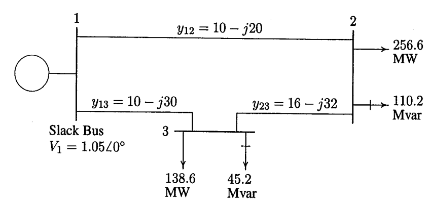
The single-line diagram of a
three-bus power system is shown below, with generation located at bus 1.
The scheduled loads at buses 2 and 3 are indicated on the diagram. The
line impedances are provided in per unit on a 100 MVA base, and the line
charging susceptances are assumed to be negligible.
Using the Gauss-Seidel method, calculate the phasor values of the
voltage at the load buses 2 and 3 (P-Q buses) to four decimal
places.
Determine the real and reactive power at the slack bus.
Compute the line flows and line losses.
Construct a power flow diagram illustrating the direction of line
flow.
At the P-Q buses, the complex loads expressed in per units
are
\[S_2^{sch} = -\dfrac{(256.6 +
j110.2)}{100} = -2.566 - j1.102 \, \text{pu}\]
\[S_3^{sch} = -\dfrac{(138.6 + j45.2)}{100}
= -1.386 - j0.452 \, \text{pu}\]
Bus 1 is taken as reference bus (slack bus). Starting from an
initial estimate of
\[\begin{aligned}
V_2^{(0)} &= 1.0 + j0.0 \quad \text{and} \quad V_3^{(0)} = 1.0 +
j0.0 \\[0.5em]
V_2^{(1)} &= \dfrac{\dfrac{P_2^{sch} - jQ_2^{sch}}{V_2^{*(0)}} +
y_{12}V_1 + y_{23}V_3^{(0)}}{y_{12}+y_{23}} \\[1em]
&= \dfrac{\dfrac{-2.566 + j1.102}{1.0 - j0} + (10 - j20)(1.05 + j0) +
(16 - j32)(1.0 + j0)}{(26-j52)} \\
&= 0.9825 - j0.0310 \, \text{pu}
\end{aligned}\]
\[\begin{aligned}
V_3^{(1)} &= \dfrac{\dfrac{P_3^{sch} - jQ_3^{sch}}{V_3^{*(0)}} +
y_{13}V_1 + y_{23}V_2^{(1)} }{y_{13}+y_{23}}\\[1em]
&= \dfrac{\dfrac{-1.386 + j0.452}{1.0 - j0} + (10 - j30)(1.05 +
j0) + (16 - j32)(0.9825 - j0.0310)}{(26-j62)} \\
&= 1.0011 - j0.0353
\end{aligned}\]
For the \(2^\text{nd}\)
iteration,
\[\begin{aligned}
V_2^{(2)} &= \dfrac{\dfrac{-2.566 + j1.102}{0.9825 + j0.0310} +
(10 - j20)(1.05 + j0) + (16 - j32)(1.0011 - j0.0353)}{(26 - j52)} \\
&= 0.9816 - j0.0520 \\
V_3^{(2)} &= \dfrac{\dfrac{-1.386 + j0.452}{1.0011 + j0.0353} +
(10 - j30)(1.05 + j0) + (16 - j32)(0.9816 - j0.052)}{(26 - j62)} \\
&= 1.0008 - j0.0459
\end{aligned}\]
The process is continued and a solution is converged with an accuracy
of \(5 \times 10^{-5}\) per unit in
seven iterations as given below.
\[\begin{aligned}
V_2^{(3)} & = 0.9808 - j0.0578 \qquad
V_3^{(3)} = 1.0004 - j0.0488 \\
V_2^{(4)} & = 0.9803 - j0.0594 \qquad
V_3^{(4)} = 1.0002 - j0.0497 \\
V_2^{(5)} & = 0.9801 - j0.0598 \qquad
V_3^{(5)} = 1.0001 - j0.0499 \\
V_2^{(6)} & = 0.9801 - j0.0599 \qquad
V_3^{(6)} = 1.0000 - j0.0500 \\
V_2^{(7)} & = 0.9800 - j0.0600 \qquad
V_3^{(7)} = 1.0000 - j0.0500
\end{aligned}\]
The final solution is
\[V_2 = 0.9800 - j0.0600 = 0.98183
\angle{-3.5035} \, \text{pu}\]
\[\begin{aligned}
P_1 - jQ_1 &= V_1^*\bigg[V_1(y_{12} + y_{13}) - (y_{12}V_2 +
y_{13}V_3)\bigg] \\
&= 1.05\bigg[1.05(20 - j50) - (10 - j20)(0.98 - j0.06) \\
&- (10 - j30)(1.0 - j0.05)\bigg] \\
&= 4.095 - j1.890
\end{aligned}\]
b)
\[P_1 = 4.095 \, \text{pu} = 409.5 \, \text{MW}
\quad \text{and} \quad Q_1 = 1.890 \, \text{pu} = 189.0 \,
\text{MVAR}.\]
or the slack bus real and reactive powers are
\[\begin{aligned}
I_{12} &= y_{12}(V_1 - V_2) \\
&= (10 - j20)\big[(1.05 + j0) - (0.98 - j0.06)\big] = 1.9 - j0.8
\\
I_{21} &= -I_{12} = -1.9 + j0.8 \\
I_{13} &= y_{13}(V_1 - V_3) \\
&= (10 - j30)\big[(1.05 + j0) - (1.0 - j0.05)\big] = 2.0 - j1.0
\\
I_{31} &= -I_{13} = -2.0 + j1.0 \\
I_{23} &= y_{23}(V_2 - V_3) \\
&= (16 - j32)\big[(0.98 - j0.06) - (1 - j0.05)\big] = -0.64 +
j0.48\\
I_{32} &= -I_{23} = 0.64 - j0.48
\end{aligned}\]
c)
The line flows are
\[\begin{aligned}
S_{12} &= V_1 I_{12}^* = (1.05 + j0.0)(1.9 + j0.8) = 1.995 +
j0.84 \, \text{pu} \\
&= \mathrm{199.5~MW} + j\mathrm{84.0~MVAR} \\
S_{21} &= V_2 I_{21}^* = (0.98 - j0.06)(-1.9 - j0.8) = -1.91 -
j0.67 \, \text{pu} \\
&= \mathrm{-191.0~MW} - j\mathrm{67.0~MVAR} \\
S_{13} &= V_1 I_{13}^* = (1.05 + j0.0)(2.0 + j1.0) = 2.1 + j1.05
\, \text{pu} \\
&= \mathrm{210.0~MW} + j\mathrm{105.0~MVAR} \\
S_{31} &= V_3 I_{31}^* = (1.0 - j0.05)(-2.0 - j1.0) = -2.05 -
j0.90 \, \text{pu} \\
&= \mathrm{-205.0~MW} - j\mathrm{90.0~MVAR} \\
S_{23} &= V_2 I_{23}^* = (0.98 - j0.06)(-0.656 + j0.48) = -0.656
- j0.432 \, \text{pu} \\
&= \mathrm{-65.6~MW} - j\mathrm{43.2~MVAR} \\
S_{32} &= V_3 I_{32}^* = (1.0 - j0.05)(0.64 + j0.48) = 0.664 +
j0.448 \, \text{pu} \\
&= \mathrm{66.4~MW} + j\mathrm{44.8~MVAR}
\end{aligned}\]
The line losses are
\[\begin{aligned}
S_{L\,12} &= S_{12} + S_{21} = \mathrm{8.5~MW} +
j\mathrm{17.0~MVAR} \\
S_{L\,13} &= S_{13} + S_{31} = \mathrm{5.0~MW} +
j\mathrm{15.0~MVAR} \\
S_{L\,23} &= S_{23} + S_{32} = \mathrm{0.8~MW} +
j\mathrm{1.60~MVAR}
\end{aligned}\]
d) The power flow diagram :