Lecture Video
SECTION 01
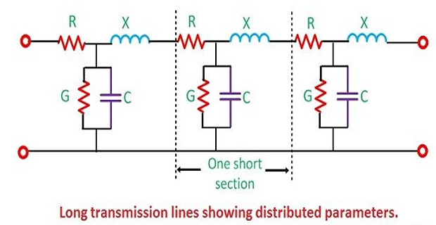
Long transmission line
TL having a length more than 240 km
Parameters are uniformly distributed along the whole length of the line.
Line may be divided into various sections, and each section consists of an inductance, capacitance, resistance and conductance
Long incremental
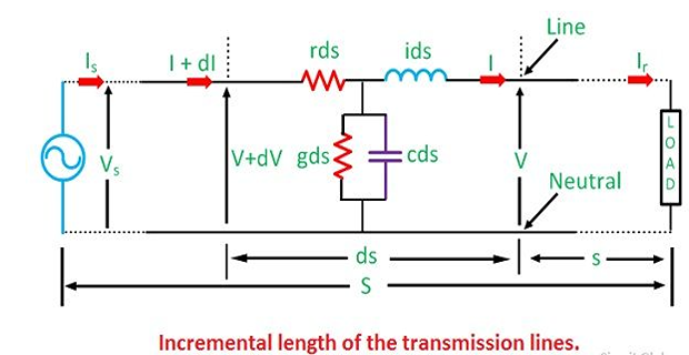
\[\begin{aligned} dV_{x} & =I_{x}zdx\Rightarrow\dfrac{dV_{x}}{dx}=zI_{x}\\ dI_{x} & =V_{x}ydx\Rightarrow\dfrac{dI_{x}}{dx}=yV_{x} \end{aligned}\]
\[\dfrac{d^{2}V_{x}}{dx^{2}}=\dfrac{dI_{x}}{dx}z=yV_{x}z\]
\[\dfrac{dV_{x}}{dx}=C_{1}\gamma e^{\gamma
x}-C_{2}\gamma e^{-\gamma x}=zI_{x}\]
\[\boxed{Z_{c}=\sqrt{\left(\dfrac{z}{y}\right)}}\]
\[\therefore I_{x}=\dfrac{C_{1}}{Z_{c}}e^{\gamma
x}-\dfrac{C_{2}}{Z_{c}}e^{-\gamma x}\]
\[\begin{aligned} V_{x}&=C_{1}e^{\gamma x}+C_{2}e^{-\gamma x}\\ I_{x}&=\dfrac{C_{1}}{Z_{c}}e^{\gamma
x}-\dfrac{C_{2}}{Z_{c}}e^{-\gamma x} \end{aligned}\]
\[\begin{aligned} V_{x} & =V_{R}\left(\dfrac{e^{\gamma x}+e^{-\gamma
x}}{2}\right)+I_{R}Z_{c}\left(\dfrac{e^{\gamma x}-e^{-\gamma
x}}{2}\right)\\ &=V_{R}cosh\left(\gamma x\right)+I_{R}Z_{c}sinh\left(\gamma
x\right) \end{aligned}\]
\[\begin{aligned} I_{x} & =V_{R}\dfrac{1}{Z_{c}}\left(\dfrac{e^{\gamma
x}-e^{-\gamma x}}{2}\right)e^{\gamma x}+I_{R}\left(\dfrac{e^{\gamma
x}+e^{-\gamma x}}{2}\right)\\ &=I_{R}cosh\left(\gamma
x\right)+V_{R}\dfrac{1}{Z_{c}}sinh\left(\gamma x\right) \end{aligned}\]
$$\boxed{
\left[\begin{array}{c}
V_S \\
I_S
\end{array}\right]=\left[\begin{array}{cc}
\cosh (\gamma l) & Z_c \sinh (\gamma l) \\
\frac{1}{Z_c} \sinh (\gamma l) & \cosh (\gamma l)
\end{array}\right]\left[\begin{array}{c}
V_R \\
I_R
\end{array}\right]
}$$
SECTION 02
Evaluation of ABCD constants of Long TL
\[\gamma=\sqrt{yz}=\alpha+j\beta\]
\[\begin{aligned}
cosh\left(\alpha l+j\beta l\right) & =cosh\left(\alpha
l\right)cos\left(\beta l\right)+jsinh\left(\alpha l\right)sin\left(\beta
l\right)\\
sinh\left(\alpha l+j\beta l\right) & =sinh\left(\alpha
l\right)cos\left(\beta l\right)+jcosh\left(\alpha l\right)sin\left(\beta
l\right)
\end{aligned}\]
The trigonometric values can be looked from standard tables.
\[\begin{aligned}
cosh\left(\gamma l\right) &
=1+\dfrac{\gamma^{2}l^{2}}{2!}+\dfrac{\gamma^{4}l^{4}}{4!}+\cdots\approx\left(1+\dfrac{YZ}{2}\right)\\
sinh\left(\gamma l\right) & =\gamma
l+\dfrac{\gamma^{3}l^{3}}{3!}+\dfrac{\gamma^{5}l^{5}}{5!}+\cdots\approx\sqrt{YZ}\left(1+\dfrac{YZ}{6}\right)
\end{aligned}\]
\[\begin{aligned}
cosh\left(\alpha l+j\beta l\right) & =\dfrac{1}{2}\left(e^{\alpha
l}\angle\beta l+e^{-\alpha l}\angle-\beta l\right)\\
sinh\left(\alpha l+j\beta l\right) & =\dfrac{1}{2}\left(e^{\alpha
l}\angle\beta l-e^{-\alpha l}\angle-\beta l\right)
\end{aligned}\]
SECTION 03
Interpretation of the long line equations
\[\gamma=\alpha+j\beta\]
| Real part \(\alpha\) : | |
| Imaginary part \(\beta\) : |
\[\begin{aligned} V_{x} & =\left|\dfrac{V_{R}+I_{R}Z_{c}}{2}\right|e^{\alpha
x}e^{j\left(\beta
x+\phi_{1}\right)}+\left|\dfrac{V_{R}-I_{R}Z_{c}}{2}\right|e^{-\alpha
x}e^{-j\left(\beta x-\phi_{2}\right)} \end{aligned}\]
Instantaneous voltage, \(v_{x}\left(t\right) =v_{x1}+v_{x2}\)
\[\begin{cases} v_{x1} &
=\sqrt{2}\left|\dfrac{V_{R}+I_{R}Z_{c}}{2}\right|e^{\alpha
x}cos\left(\omega t+\beta x+\phi_{1}\right)\\ v_{x2} &
=\sqrt{2}\left|\dfrac{V_{R}-I_{R}Z_{c}}{2}\right|e^{-\alpha
x}cos\left(\omega t-\beta x+\phi_{2}\right) \end{cases}\]
\[\begin{aligned}
\phi_{1} & = \angle\left(V_{R}+I_{R}Z_{c}\right)\\
\phi_{2} & = \angle\left(V_{R}-I_{R}Z_{c}\right)
\end{aligned}\]
\(v_{x}\left(t\right)\) is a function of two variables - time & distance
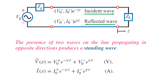
Represents two travelling waves: Incident and reflected waves
Incident reflected