SECTION 01
Newton-Raphson Method
\[\begin{aligned}
f_{1}\left(x_{1},\cdots,x_{n}\right) & =\eta_{1}\\
f_{2}\left(x_{1},\cdots,x_{n}\right) & =\eta_{2}\\
\vdots\\
f_{n}\left(x_{1},\cdots,x_{n}\right) & =\eta_{n}
\end{aligned}\]
\[\begin{aligned}
g_{1}\left(x_{1},\cdots,x_{n}\right) &
=f_{1}\left(x_{1},\cdots,x_{n}\right)-\eta_{1}=0\\
g_{2}\left(x_{1},\cdots,x_{n}\right) &
=f_{2}\left(x_{1},\cdots,x_{n}\right)-\eta_{2}=0\\
& \vdots\\
g_{n}\left(x_{1},\cdots,x_{n}\right) &
=f_{n}\left(x_{1},\cdots,x_{n}\right)-\eta_{n}=0
\end{aligned}\]
\[\begin{aligned}
x_{1}^{*} & =x_{1}^{(0)}+\varDelta x_{1}^{(0)}\\
x_{2}^{*} & =x_{2}^{(0)}+\varDelta x_{2}^{(0)}\\
& \vdots\\
x_{n}^{*} & =x_{n}^{(0)}+\varDelta x_{n}^{(0)}
\end{aligned}\]
to get correct solution of these
variables and add corrections variables as Assume initial estimates of the
\[g_{k}\left(x_{1}^{*},\cdots,x_{n}^{*}\right)=g_{k}\left(x_{1}^{(0)}+\varDelta
x_{1}^{(0)},\cdots x_{n}^{(0)}+\varDelta x_{n}^{(0)}\right)=0,\]
\[ \begin{aligned}
g_{k}\left(x_{1}^{*},\cdots,x_{n}^{*}\right)=g_{k}\left(x_{1}^{(0)},\cdots,x_{n}^{(0)}\right)+\varDelta
x_{1}^{(0)}\left.\dfrac{\partial g_{k}}{\partial
x_{1}}\right|^{(0)}+\varDelta x_{2}^{(0)}\left.\dfrac{\partial
g_{k}}{\partial x_{2}}\right|^{(0)}+\cdots+\varDelta
x_{n}^{(0)}\left.\dfrac{\partial g_{k}}{\partial x_{n}}\right|^{(0)}
\end{aligned}
\]
\[\left[\begin{array}{cccc}
\dfrac{\partial g_{1}}{\partial x_{1}} & \dfrac{\partial
g_{1}}{\partial x_{2}} & \cdots & \dfrac{\partial
g_{1}}{\partial x_{n}}\\
\dfrac{\partial g_{2}}{\partial x_{1}} & \dfrac{\partial
g_{2}}{\partial x_{2}} & \cdots & \dfrac{\partial
g_{2}}{\partial x_{n}}\\
\vdots & \vdots & \ddots & \vdots\\
\dfrac{\partial g_{n}}{\partial x_{1}} & \dfrac{\partial
g_{n}}{\partial x_{2}} & & \dfrac{\partial g_{n}}{\partial
x_{n}}
\end{array}\right]^{\left(0\right)}\left[\begin{array}{c}
\varDelta x_{1}^{(0)}\\
\varDelta x_{2}^{(0)}\\
\vdots\\
\varDelta x_{n}^{(0)}
\end{array}\right]=\left[\begin{array}{c}
0-g_{1}\left(x_{1}^{(0)},\cdots,x_{n}^{(0)}\right)\\
0-g_{2}\left(x_{1}^{(0)},\cdots,x_{n}^{(0)}\right)\\
\vdots\\
0-g_{n}\left(x_{1}^{(0)},\cdots,x_{n}^{(0)}\right)
\end{array}\right]\]
\(J\)
Jacobian
matrix Equation can be written in vector-matrix form as
\[\left[\begin{array}{c}
\varDelta x_{1}^{(0)}\\
\varDelta x_{2}^{(0)}\\
\vdots\\
\varDelta x_{n}^{(0)}
\end{array}\right]=\left[J^{\left(0\right)}\right]^{-1}\left[\begin{array}{c}
\varDelta g_{1}^{(0)}\\
\varDelta g_{2}^{(0)}\\
\vdots\\
\varDelta g_{n}^{(0)}
\end{array}\right]\]
Taylor ’s series is truncated by neglecting the 2nd and higher
order terms, we cannot expect to find the correct solution at the end of
first iteration. We shall then have
\[\begin{aligned}
x_{1}^{(1)} & =x_{1}^{(0)}+\varDelta x_{1}^{(0)}\\
x_{2}^{(1)} & =x_{2}^{(0)}+\varDelta x_{2}^{(0)}\\
& \vdots\\
x_{n}^{(1)} & =x_{n}^{(0)}+\varDelta x_{n}^{(0)}
\end{aligned}\]
These are then used to find \(J^{(1)}\) and \(\varDelta g_k^{(1)},~ k = 1,\cdots , n\)
.
We can then find \(\varDelta x_2^{(1)}
, \cdots , \varDelta x_n^{(1)}\) and subsequently calculate \(x_2^{(1)}, \cdots , x_n^{(1)}\).
The process continues till \(\varDelta
g_k,~ k = 1, \cdots , n\) becomes less than a small
quantity.
SECTION 02
Load Flow By Newton-Raphson Method
At each iteration form a Jacobian matrix and solve for the
corrections
\[J=\left[\begin{array}{cc}
J_{11} & J_{12}\\
J_{21} & J_{22}
\end{array}\right]\]
The Jacobian matrix is divided into sub-matrices as
\[\left(n + n_p -1\right) \times \left(n +
n_p -1\right)\]
\[\begin{array}{cc}
J_{11}: & \left(n-1\right)\times\left(n-1\right)\\
J_{12}: & \left(n-1\right)\times n_{p}\\
J_{21}: & n_{p}\times\left(n-1\right)\\
J_{22}: & n_{p}\times n_{p}
\end{array}\]
Dimensions of the sub-matrices are as follows
\[ \begin{aligned}
J_{11} & =\left[\begin{array}{ccc}
\dfrac{\partial P_{2}}{\partial\delta_{2}} & \cdots &
\dfrac{\partial P_{2}}{\partial\delta_{n}}\\
\vdots & \ddots\\
\dfrac{\partial P_{n}}{\partial\delta_{2}} & & \dfrac{\partial
P_{n}}{\partial\delta_{n}}
\end{array}\right]~~~~~~~J_{12}=\left[\begin{array}{ccc}
\left|V_{2}\right|\dfrac{\partial P_{2}}{\partial\left|V_{2}\right|}
& \cdots & \left|V_{1+n_{p}}\right|\dfrac{\partial
P_{2}}{\partial\left|V_{1+n_{p}}\right|}\\
\vdots & \ddots\\
\left|V_{2}\right|\dfrac{\partial P_{n}}{\partial\left|V_{2}\right|}
& \cdots & \left|V_{1+n_{p}}\right|\dfrac{\partial
P_{n}}{\partial\left|V_{1+n_{p}}\right|}
\end{array}\right]\\
J_{21} & =\left[\begin{array}{ccc}
\dfrac{\partial Q_{2}}{\partial\delta_{2}} & \cdots &
\dfrac{\partial Q_{2}}{\partial\delta_{n}}\\
\vdots & \ddots\\
\dfrac{\partial Q_{1+n_{p}}}{\partial\delta_{2}} & \cdots &
\dfrac{\partial Q_{1+n_{p}}}{\partial\delta_{n}}
\end{array}\right]\:J_{22}=\left[\begin{array}{ccc}
\left|V_{2}\right|\dfrac{\partial Q_{2}}{\partial\left|V_{2}\right|}
& \cdots & \left|V_{1+n_{p}}\right|\dfrac{\partial
Q_{2}}{\partial\left|V_{1+n_{p}}\right|}\\
\vdots & \ddots\\
\left|V_{2}\right|\dfrac{\partial
Q_{1+n_{p}}}{\partial\left|V_{2}\right|} & \cdots &
\left|V_{1+n_{p}}\right|\dfrac{\partial
Q_{1+n_{p}}}{\partial\left|V_{1+n_{p}}\right|}
\end{array}\right]
\end{aligned}
\]
SECTION 03
Load Flow Algorithm
The Newton-Raphson procedure is as follows:
Choose the initial values of the voltage magnitudes \(\left|V\right|^{(0)}\) for all \(n_p\) load buses and \(n-1\) angles \(\delta^{(0)}\) of the voltages of all the
buses except the slack bus
Use the estimated \(\left|V\right|^{(0)}\) and \(\delta^{(0)}\) to calculate a total \(n-1\) number of injected real power \(P_{calc}^{(0)}\) and equal number of real
power mismatch \(\varDelta
P^{(0)}\)
Use the estimated \(\left|V\right|^{(0)}\) and \(\delta^{(0)}\) to calculate a total \(n_p\) number of injected reactive power
\(Q_{calc}^{(0)}\) and equal number of
reactive power mismatch \(\varDelta
Q^{(0)}\)
Use the estimated \(\left|V\right|^{(0)}\) and \(\delta^{(0)}\) to form the Jacobian matrix
\(J^{(0)}\)
Solve equation for \(\delta^{(0)}\)
and \(\varDelta \left|V\right|^{(0)} \div
\left|V\right|^{(0)}\)
Obtain the updates
\[\begin{aligned} \delta^{(1)} & =\delta^{(0)}+\varDelta\delta^{(0)}\\ \left|V\right|^{(1)} &
=\left|V\right|^{(0)}\left[1+\dfrac{\varDelta\left|V\right|^{(0)}}{\left|V\right|^{(0)}}\right] \end{aligned}\]
Check if all the mismatches are below a small number. Terminate the
process if yes. Otherwise go back to step-1 to start the next
iteration
Formation of \(J_{11}\)
\[J_{11}=\left[\begin{array}{ccc}
L_{22} & \cdots & L_{2n}\\
\vdots & \ddots & \vdots\\
L_{n2} & \cdots & L_{nn}
\end{array}\right]\]
\[\begin{aligned}
L_{ik} & =\dfrac{\partial
P_{i}}{\partial\delta_{k}}=-\left|Y_{ik}V_{i}V_{k}\right|sin\left(\theta_{ik}+\delta_{k}-\delta_{i}\right),~i\neq
k\\
L_{ii} & =\dfrac{\partial
P_{i}}{\partial\delta_{i}}=\sum_{\begin{array}{c} k=1\\ k\neq i \end{array}}^{n}\left|Y_{ik}V_{i}V_{k}\right|sin\left(\theta_{ik}+\delta_{k}-\delta_{i}\right)\\
& =-Q_{i}-\left|V_{i}\right|^{2}B_{ii}
\end{aligned}\]
Formation of \(J_{21}\)
\[J_{21}=\left[\begin{array}{ccc}
M_{22} & \cdots & M_{2n}\\
\vdots & \ddots & \vdots\\
M_{n2} & \cdots & M_{nn}
\end{array}\right]\]
\[J_{12}=\left[\begin{array}{ccc}
N_{22} & \cdots & N_{2n}\\
\vdots & \ddots & \vdots\\
N_{n2} & \cdots & N_{nn}
\end{array}\right]\]
Formation of \(J_{12}\)
\[J_{22}=\left[\begin{array}{ccc}
O_{22} & \cdots & O_{2n}\\
\vdots & \ddots & \vdots\\
O_{n2} & \cdots & O_{nn}
\end{array}\right]\]
Formation of \(J_{22}\)
SECTION 05
Solution of Newton-Raphson Load Flow
\[ \begin{aligned}
L_{23}^{(0)} &
=-\left|Y_{23}V_{2}^{(0)}V_{3}^{(0)}\right|sin\left(\theta_{23}+\delta_{3}-\delta_{2}\right)\\
&=-\left|Y_{23}\right|sin\theta_{23}=-B_{23}=-4.8077\\
Q_{2}^{(0)} & =-\left|V_{2}^{(0)}\right|^{2}B_{22}-{\displaystyle
\sum_{\begin{array}{c} k=1\\ k\neq2 \end{array}}^{n}\left|Y_{2k}V_{2}^{(0)}V_{k}^{(0)}\right|sin\left(\theta_{2k}+\delta_{k}-\delta_{2}\right)}\\
& =-B_{22}-1.05B_{21}-B_{23}-B_{24}-1.02B_{25}=-0.6327\\
L_{22}^{(0)} &
=-Q_{2}^{(0)}-\left|V_{2}^{(0)}\right|^{2}B_{22}=-0.6327-B_{22}=18.8269
\end{aligned}
\]
\[J_{11}^{(0)}=\left[\begin{array}{cccc}
18.8269 & -4.8077 & 0 & -3.9231\\
-4.8077 & 11.1058 & -3.8462 & -2.4519\\
0 & -3.8462 & 5.8077 & -1.9615\\
-3.9231 & -2.4519 & -1.9615 & 12.4558
\end{array}\right]\]
\[
J_{21}=M\left(1:3,1:4\right)~and~J_{12}=-M\left(1:4,1:3\right)\Longleftarrow
M=\left[\begin{array}{cccc}
M_{11} & M_{12} & M_{13} & M_{14}\\
M_{21} & M_{22} & M_{23} & M_{24}\\
M_{31} & M_{32} & M_{33} & M_{34}\\
M_{41} & M_{42} & M_{43} & M_{44}
\end{array}\right]
\]
\[J_{21}^{(0)}=\left[\begin{array}{cccc}
-3.7654 & 0.9615 & 0 & 0.7846\\
0.9615 & -2.2212 & 0.7692 & 0.4904\\
0 & 0.7692 & -1.1615 & 0.3923
\end{array}\right]\]
\[J_{12}^{(0)}=\left[\begin{array}{ccc}
3.5423 & -0.9615 & 0\\
-0.9615 & 2.2019 & -0.7692\\
0 & -0.7692 & 1.1462\\
0.7846 & -0.4904 & -0.3923
\end{array}\right]\]
\[J_{22}^{(0)}=\left[\begin{array}{ccc}
17.5615 & -4.8077 & 0\\
-4.8077 & 10.8996 & -3.8462\\
0 & -3.8462 & 5.5408
\end{array}\right]\]
\[\begin{aligned}
P_{calc}^{(0)} & =\left[\begin{array}{cccc}
-0.1115 & -0.0096 & -0.0077 &
-0.0098\end{array}\right]^{T}\\
Q_{calc}^{(0)} & =\left[\begin{array}{ccc}
-0.6327 & -0.1031 & -0.1335\end{array}\right]^{T}
\end{aligned}\]
\[\begin{aligned}
\varDelta P^{(0)} & =\left[\begin{array}{cccc}
-0.8485 & -0.3404 & -0.1523 & 0.2302\end{array}\right]^{T}\\
\varDelta Q^{(0)} & =\left[\begin{array}{ccc}
0.0127 & -0.0369 & 0.0535\end{array}\right]^{T}
\end{aligned}\]
From the initial conditions the power and reactive power are computed
as
\[\left[\begin{array}{c}
\delta_{2}^{(0)}\\
\delta_{3}^{(0)}\\
\delta_{4}^{(0)}\\
\delta_{5}^{(0)}
\end{array}\right]=\left[\begin{array}{c}
-4.91\\
-6.95\\
-7.19\\
-3.09
\end{array}\right]deg~~\left[\begin{array}{c}
\left|V_{2}\right|^{(0)}\\
\left|V_{3}\right|^{(0)}\\
\left|V_{4}\right|^{(0)}
\end{array}\right]=\left[\begin{array}{c}
0.9864\\
0.9817\\
0.9913
\end{array}\right]\]
\(10^{-6}\)\(\varDelta Q\)\(\varDelta P\)Then the updates at the end of the first iteration are given as
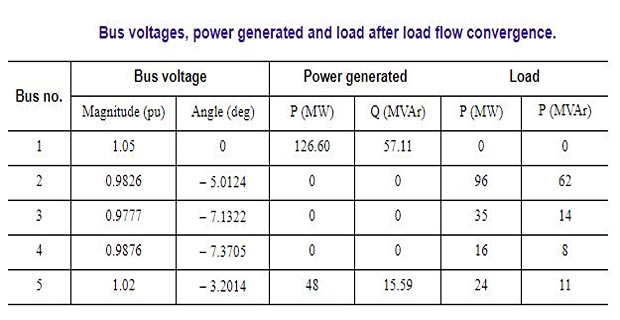
SECTION 06
Load Flow Results Conclusions
Both GS and NR methods yields the same result
However NR method converged faster than the GS method
Total power generated = 174.6 MW whereas total load = 171
MW
Line loss = 3.6 MW for all the lines put together
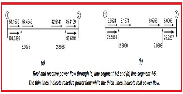
\[\begin{aligned}
I_{12} & =0.9623-j0.5187=1.0932\angle-28.33^{0}~pu\\
S_{12} & =V_{1}I_{12}^{*}\times100=-101.0395-j54.4645~MW\\
S_{21} & =V_{2}I_{12}^{*}\times100=98.6494+j42.5141~MW
\end{aligned}\]
-ve sign in power indicates the power is leaving the bus (leaving the
bus-1 and entering the bus-2)
out of a total amount of 101.0395 MW of real power dispatched
from bus-1 over the line segment 1-2, 98.6494 MW reaches bus-2. This
indicates that the drop in the line segment is 2.3901 MW.
\[\begin{aligned}
\left|I_{12}\right|^{2}\times R_{12}\times100 &
=1.0932^{2}\times0.02\times100=2.3901~MW\\
\left|I_{12}\right|^{2}\times X_{12}\times100 &
=1.0932^{2}\times0.1\times100=10.9508~MVAr
\end{aligned}\]
Also, \(I^2X\) loss can be
calculated by subtracting the reactive power absorbed by bus-2 from that
supplied by bus-1
The above calculation however does not include the line
charging
Since the line is modelled by an equivalent-\(\pi\), the voltage across the shunt
capacitor is the bus voltage to which the shunt capacitor is
connected
Therefore the current flowing through line segment is not the
current leaving bus-1 or entering bus-2
It is the current flowing in between the two charging
capacitors
Since the shunt branches are purely reactive, the real power flow
does not get affected by the charging capacitors
Each charging capacitor is assumed to inject a reactive power
that is the product of the half line charging admittance and square of
the magnitude of the voltage of that at bus