Overview
Lecture-12: Capacitance of Single-Phase TL
Lecture-13: Capacitance of a Three-Phase TL
Lecture-14: Effect of Earth on Capacitance of the TL
Lecture-15: Capacitance Calculations for Bundle Conductors
Introduction to Capacitance of a TL
Due to potential difference between the conductor
\[C = \dfrac{q}{V}\]Gauss’s law for electric field:
total \(q\) within a closed surface equal total electric flux emerging from the surface
Between parallel conductors
\(C\) is a constant
depends on the size and spacing of the conductors
Power lines less than 80 Km \(\Longrightarrow\) \(C\) is slight and neglected
For longer HV lines \(C\) becomes important
AC voltage \(\Longrightarrow\) charge \(\Longrightarrow\) Charging current \((I_c)\)
\(I_c\) flows even when the TL is open-circuited
affects the voltage drop along the lines
Efficiency and power factor
Stability of the system
Electric field of a long straight conductor
If the conductor lies in uniform medium such as air and isolated from other charges then \(q\) is uniformly distributed around its periphery and the flux is radial
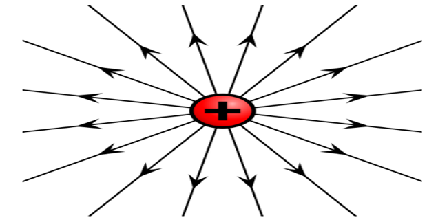
- m from the conductor: flux leaving the conductor per m of length divided by the area of the surface in an axial length of 1m The electric flux density at\[D_f = \dfrac{q}{2 \pi x}~C/m^2\]
- \(\epsilon =\)\[E = \dfrac{q}{2 \pi x \epsilon}~V/m\]
\(q =\)The electric field intensity
Potential difference between two points due to a charge
\(V = W/q\) and \(E = F/q\)
\(+ve\) charge on the conductor exerts a repelling force on a \(+ve\) charge placed in the field
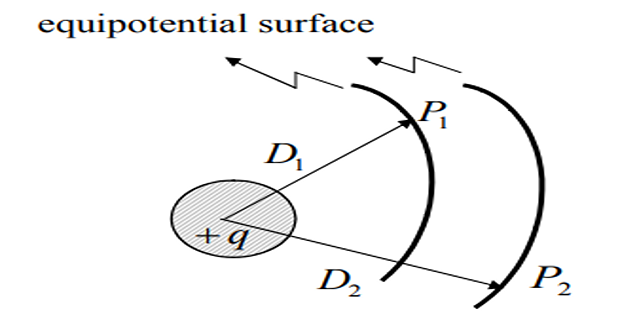
\(P_1\) is at higher potential than \(P_2\)
work must be done to move from \(P_2\) to \(P_1\)
- and Instantaneous voltage drop between\[v_{12}=\intop_{D_{1}}^{D_{2}}E\cdot dx=\intop_{D_{1}}^{D_{2}}\dfrac{q}{2\pi\varepsilon x}\cdot dx=\dfrac{q}{2\pi\varepsilon}ln\dfrac{D_{2}}{D_{1}}~V\]
Voltage drop may be +ve or -ve, depends on
\(q\) is +ve or -ve
voltage drop is computed near to far or vice versa
Capacitance of a two-wire line
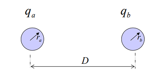
- is the sum of each charge on the conductor alone to By principle of superposition the voltage drop from\[v_{ab}=\begin{array}{c} \underbrace{\dfrac{q_{a}}{2\pi\varepsilon}ln\dfrac{D}{r_{a}}}\\ \mbox{due to }q_{a} \end{array}+\begin{array}{c} \underbrace{\dfrac{q_{b}}{2\pi\varepsilon}ln\dfrac{r_{b}}{D}}\\ \mbox{due to }q_{b} \end{array}~V\]
- for a two-wire line Since,\[v_{ab} =\dfrac{q_{a}}{2\pi\varepsilon}\left(ln\dfrac{D}{r_{a}}-ln\dfrac{r_{b}}{D}\right)=\dfrac{q_{a}}{2\pi\varepsilon}ln\dfrac{D^{2}}{r_{a}r_{b}}~V\]
- The capacitance between conductors\[C_{ab}=\dfrac{q_{a}}{V_{ab}}=\dfrac{2\pi\varepsilon}{ln\left(D^{2}/r_{a}r_{b}\right)}~F/m\]
If \(r_{a}=r_{b}=r\)
equation* C_ab= F/m
equation* C_n=C_an=C_bn== F/m
NOTE: \(r\) used in \(C\) calculation is actual radius of the conductor, unlike use of GMR in \(L\)
- The capacitive reactance between one conductor and neutral\[X_{c}=\dfrac{1}{2\pi fC_{n}}=\dfrac{2.862}{f}\times10^{9}ln\dfrac{D}{r}~\Omega m\]