Demonstrative Video
Resonance
Feature of the frequency response of a circuit \(\Rightarrow\) sharp peak (or resonant peak) exhibited in its amplitude characteristic.
System that has a complex conjugate pair of poles; cause of oscillations of stored energy from one form to another.
Allows frequency discrimination in communications networks.
Occurs in any circuit that has at least one \(L\) and one \(C\).
Resonance : condition in an RLC circuit in which the \(|X_C|= |X_L|\), thereby resulting in a purely resistive impedance.
Resonant circuits (series or parallel) are useful for constructing filters, as their TFs can be highly frequency selective.
Used in many applications such as selecting the desired stations in radio and TV receivers.
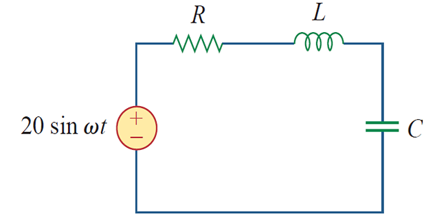
Series Resonance
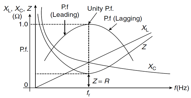
Resonant frequency \(\omega_0\) : at which \(\mathbf{Z}\) of the circuit is purely real
At resonance:
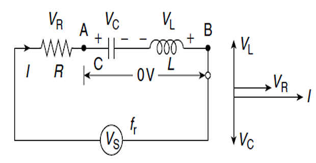
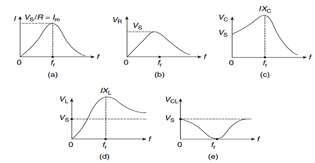
\(\mathbf{Z} = R~\Rightarrow\) \(LC\) series acts as SC and the entire \(\mathbf{V_s}\) is across \(R\)
\(\mathbf{V_s}\) and \(\mathbf{I}\) in phase \(\Rightarrow\) PF is unity
\(\mathbf{H(\omega)} = \mathbf{Z(\omega)}\) minimum
- is Quality factor \(\mathbf{V_s}\)\(\mathbf{V_C}\)\(\mathbf{V_L}\)\[\begin{aligned} \left|\mathbf{V}_{L}\right| &=\frac{V_{m}}{R} \omega_{0} L=Q V_{m} \\ \left|\mathbf{V}_{C}\right| &=\frac{V_{m}}{R} \frac{1}{\omega_{0} C}=Q V_{m} \end{aligned}\]
series resonant circuit also called voltage resonant
circuit
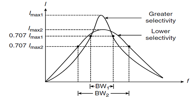
At certain \(\omega = \omega_1, \omega_2\) the dissipated power is half the max. value.
Known as Half-power frequencies
- Resonant frequency is the geometric mean of the half-power frequencies\[\omega_0 = \sqrt{\omega_1 \cdot \omega_2}\]
\(\omega_1, \omega_2\) are not symmetrical around \(\omega_0\) because frequency response is not symmetrical, however it is often a reasonable approximation
- \(B\)width\(R\)Height\[\textbf{Bandwidth}~B = \omega_2 - \omega_1\]
Quality factor : Quantitate measurement of the sharpness of the resonance in a resonance circuit
\[Q=2 \pi \frac{\text { Peak energy stored in the circuit }}{\begin{array}{c} \text { Energy dissipated by the circuit } \\ \text { in one period at resonance } \end{array}}\]
\(\boxed{Q~\uparrow~\Rightarrow~B~\downarrow}\)
\(Q\) of a resonant circuit is the ratio of its \(\omega_0\) to its \(B\)
RLC circuit selectivity is the ability to respond to a certain frequency and discriminate against all other frequencies.
Frequency band to be selected or rejected is narrow, \(Q\) must be high.
If the band of frequencies is wide, \(Q\) must be low.
High-\(Q\) circuits \(\Rightarrow\) \(Q \geq 10\)
- For all practical purpose\[\omega_{1} \simeq \omega_{0}-\frac{B}{2}, \quad \omega_{2} \simeq \omega_{0}+\frac{B}{2}\]
High-Q circuits are used often in communications networks
Resonant circuit is characterized by five related parameters: \(\omega_0, \omega_1, \omega_2, Q, B\)
Problem
Given: \(R=2~\Omega,~L=1~\mathrm{mH},~C=0.4~\mathrm{\mu F}\). Determine
\(\omega_{0}, ~\omega_{1,2},~Q, ~B\)
Amplitude of the current at \(\omega_0, \omega_1, \omega_2\)