Demonstrative Video
Introduction
RLC analysis: Differential Equation (Time-domain) and Phasors (Frequency domain)
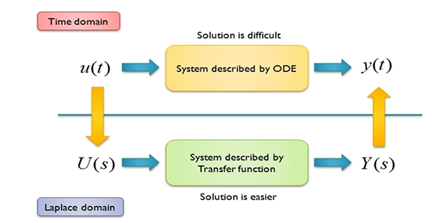
Laplace Transform : Differential Equation \(\Rightarrow\) Algebraic Equation
- Conversion Process\[\mbox{Time-domain } \mathrel{\mathop{\rightleftarrows}^{\mathrm{{\color{red}{\textbf{Laplace}}}}}_{\mathrm{{\color{brown}{\textbf{Inverse-Laplace}}}}}} \mbox{Frequency-domain}\]
Advantages of Laplace-Transform:
can be applied to a wider variety of inputs than phasor analysis
provides an easy way to solve circuit problems involving initial conditions, since it work with algebraic equations instead of DE
capable of providing one single operation, the total response of the circuit comprising both the natural and forced responses.
Definition of the Laplace Transform
Laplace transform is an integral transformation of \(f (t )\) from the time domain into the complex frequency domain, giving \(F (s)\).
- Mathematical definition\[\boxed{\mathcal{L}[f(t)]=F(s)=\int_{0^{-}}^{\infty} f(t) e^{-s t} d t} \quad s=\sigma+j \omega ~~ \text{ complex variable}\]
Argument \(st\) of \(e\) \(\Rightarrow\) dimensionless \(\Rightarrow\) unit of \(s\) is frequency or \(\mathrm{s}^{-1}\)
Lower limit \(0^{-1}\) to include origin and capture any discontinuity in \(f(t)\) at \(t=0\)
Definite integral \(\Rightarrow\) result independent of time \(\Rightarrow\) only involve \(s\)
One sided (or Unilateral)LT: Ignore for \(t < 0\) \(\Rightarrow\) \(f(t)u(t);~t \geq 0\)
- ) LT: Two-sided (or\[F(s)=\int_{-\infty}^{\infty} f(t) e^{-s t} d t\]
One-sided LT will be adequate for circuit analysis
A \(f(t)\) may not have the Laplace transform
To have a LT of \(f(t)\) the integral must converge to finite value
- , integral converges when for some Since\[\int_{0^{-}}^{\infty} e^{-\sigma t}|f(t)| d t<\infty \quad \text{for}~ \sigma = \sigma_c\]
- Region of convergence:\[\mathrm{Re}(s) = \sigma > \sigma_c \Rightarrow |F(s)| < \infty\]
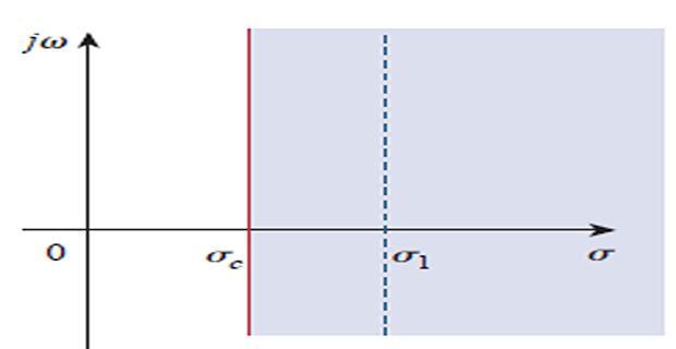
\(F(s)\) is undefined outside the region of convergence
- Inverse Laplace-transform:\[\mathcal{L}^{-1}[F(s)]=f(t)=\frac{1}{2 \pi j} \int_{\sigma_{1}-j \omega}^{\sigma_{1}+j \omega} F(s) e^{s t} d s\]
Problem
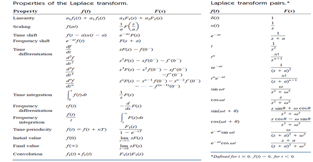
Properties of the Laplace Transform
- Linearity\[ \mathcal{L}\left[a_{1} f_{1}(t)+a_{2} f_{2}(t)\right]=a_{1} F_{1}(s)+a_{2} F_{2}(s) \]
- Scaling\[\mathcal{L}[f(a t)]=\frac{1}{a} F\left(\frac{s}{a}\right)\]
- Time Shift\[\mathcal{L}[f(t-a) u(t-a)]=e^{-a s} F(s)\]
- Frequency Shift\[\mathcal{L}\left[e^{-a t} f(t) u(t)\right]=F(s+a)\]
- Time Differentiation\[ \begin{aligned} \mathcal{L}\left[\frac{d^{n} f}{d t^{n}}\right]=& s^{n} F(s)-s^{n-1} f\left(0^{-}\right) \\ &-s^{n-2} f^{\prime}\left(0^{-}\right)-\cdots-s^{0} f^{(n-1)}\left(0^{-}\right) \end{aligned} \]
- Time Integration\[\mathcal{L}\left[\int_{0}^{t} f(t) d t\right]=\frac{1}{s} F(s)\]
- Initial and Final values\[\begin{aligned} &f(0)=\lim _{s \rightarrow \infty} s F(s) \\ &f(\infty)=\lim _{s \rightarrow 0} s F(s) \end{aligned}\]
Problems
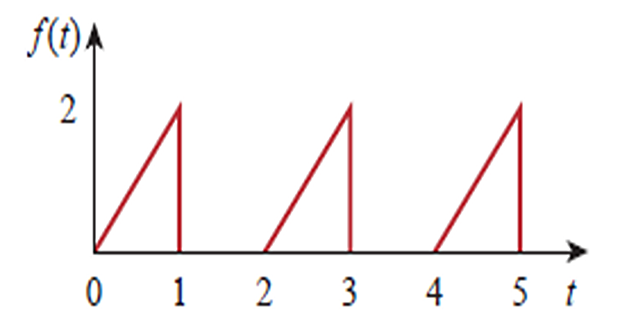
Problem-1
Find the Laplace transform of \(f(t)\) ?
Problem-2