Demonstrative Video
The Convolution Integral
Convolution (means folding) is a tool for viewing and characterizing physical systems.
- \(h(t)\)\(x(t)\)\(y(t)\)Convolution integral:\[\begin{aligned} y(t)& =\int_{-\infty}^{\infty} x(\lambda) h(t-\lambda) d \lambda \quad \Rightarrow y(t)=x(t) * h(t) \\ \lambda & \rightarrow \text{dummy variable} \quad \text{asterisk} \rightarrow \text{convolution} \end{aligned}\]
- The convolution process is commutative:\[\begin{aligned} &y(t)=x(t) * h(t)=h(t) * x(t) \\ &y(t)=\int_{-\infty}^{\infty} x(\lambda) h(t-\lambda) d \lambda=\int_{-\infty}^{\infty} h(\lambda) x(t-\lambda) d \lambda \end{aligned}\]
The order in which the two functions are convolved is immaterial
The convolution of two signals consists of time-reversing one of the signals, shifting it, and multiplying it point by point with the second signal, and integrating the product.
Simplified case:
- \(t<0\)\(x(t)=0\)Case-1:\[\begin{aligned} &y(t)=\int_{-\infty}^{\infty} x(\lambda) h(t-\lambda) d \lambda=\int_{0}^{\infty} x(\lambda) h(t-\lambda) d \lambda \end{aligned}\]
- \(\lambda > t\)\((t-\lambda) < 0\)\(h(t-\lambda)=0\)\(\Rightarrow\)\(t<0\)causal system\(h(t)=0\)Case-2:\[\begin{aligned} &\boxed{y(t)=h(t) * x(t)=\int_{0}^{t} x(\lambda) h(t-\lambda) d \lambda} \end{aligned}\]
Properties of the Convolution Integral
\(x(t) * h(t)=h(t) * x(t)\) (Commutative)
\(f(t) *[x(t)+y(t)]=f(t) * x(t)+f(t) * y(t)\) (Distributive)
\(f(t) *[x(t) * y(t)]=[f(t) * x(t)] * y(t)\) (Associative)
\(f(t) * \delta(t)=\int_{-\infty}^{\infty} f(\lambda) \delta(t-\lambda) d \lambda=f(t)\)
\(f(t) * \delta\left(t-t_{o}\right)=f\left(t-t_{o}\right)\)
\(f(t) * \delta^{\prime}(t)=\int_{-\infty}^{\infty} f(\lambda) \delta^{\prime}(t-\lambda) d \lambda=f^{\prime}(t)\)
\(f(t) * u(t)=\int_{-\infty}^{\infty} f(\lambda) u(t-\lambda) d \lambda=\int_{-\infty}^{t} f(\lambda) d \lambda\)
- Link between Laplace transform and convolution integral:\[\begin{aligned} &f(t)=f_{1}(t) * f_{2}(t)=\int_{0}^{t} f_{1}(\lambda) f_{2}(t-\lambda) d \lambda \\ &F(s)=\boxed{\mathcal{L}\left[f_{1}(t) * f_{2}(t)\right]=F_{1}(s) F_{2}(s)} \end{aligned}\]
This indicates that convolution in the time domain is equivalent to multiplication in the s-domain
Convolution in some cases is better in time-domain only
Product \(F_1(s) \cdot F_2(s)\) is very complicated finding inverse is difficult
\(f_1(t)\) and \(f_2(t)\) available in experimental data and there is no explicit Laplace transform
The process of convolving two signals in the time domain is better appreciated from a graphical point of view
Steps: graphical procedure for evaluating the convolution integral
Folding: Take the mirror image of \(h(\lambda)\) about the ordinate axis to obtain \(h(-\lambda)\).
Displacement: Shift or delay \(h(-\lambda)\) by \(t\) to obtain \(h(t-\lambda)\).
Multiplication: Find the product of \(h(t-\lambda)\) and \(x(\lambda)\).
Integration: For a given time \(t\), calculate the area under the product \(h(t-\lambda) x(\lambda)\) for \(0<\lambda<t\) to get \(y(t)\) at \(t\).
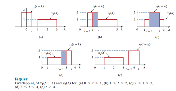
Problem
Find the convolution of the two signals ?
Solution:
Four steps to get \(y(t) = x_1(t)*x_2(t)\)
Fold \(x_1(t)\) and shift it by \(t\)
For different \(t\), multiply the two functions and integrate to determine overlapping area


Problem


