Master Bode Plots: Visualize and Analyze Circuit Frequency Response

Demonstrative Video

Bode Plots : Magnitude & Phase

\[ \begin{aligned} \mathbf{H} & = H \angle \phi = H e^{j\phi} \\ \ln \mathbf{H} & = \ln H + \ln e^{j\phi} = \underbrace{\ln (H)}_{\substack{\text{Real} \\ \text{Magnitude}}} + ~ j \underbrace{\phi}_{\substack{\text{Imaginary} \\ \text{Phase}}} \end{aligned} \]

\[ \text{Gain} ~ \boxed{H_{\mathrm{dB}} = 20 \log_{10}H} \\ \]

Both magnitude and phase plots are made on semilog graph paper.
Magnitude plot : dB Vs frequency
Phase plot : degree Vs frequency

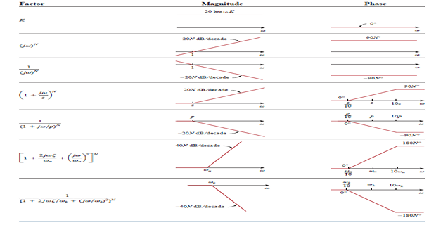
Standard form of representation of TF

\[\mathbf{H}(\omega)=\frac{K(j \omega)^{\pm 1}\left(1+j \omega / z_{1}\right)\left[1+j 2 \zeta_{1} \omega / \omega_{k}+\left(j \omega / \omega_{k}\right)^{2}\right] \cdots}{\left(1+j \omega / p_{1}\right)\left[1+j 2 \zeta_{2} \omega / \omega_{n}+\left(j \omega / \omega_{n}\right)^{2}\right] \cdots}\]

A gain \(K\)
A pole \((j \omega)^{-1}\) or zero \((j \omega)\) at the origin
A simple pole \(1 /\left(1+j \omega / p_{1}\right)\) or zero \(\left(1+j \omega / z_{1}\right)\)
A quadratic pole \(1 /\left[1+j 2 \zeta_{2} \omega / \omega_{n}+\left(j \omega / \omega_{n}\right)^{2}\right]\) or zero \(\left[1+j 2 \zeta_{1} \omega / \omega_{k}+\left(j \omega / \omega_{k}\right)^{2}\right]\)

Each factor is plotted separately and then add them graphically.
Factors are considered one at a time and then combined additively as logarithms involved.
Logarithm mathematical convenience makes Bode plots a powerful engineering tool.

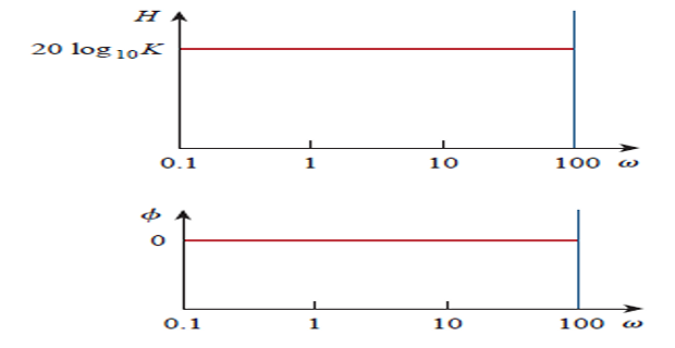
Gain \(K\):

Magnitude is \(20\log_{10}K\) and phase is \(0^{\circ}\), both constant with frequency
If \(K\) is negative, the magnitude remains same but the phase is \(\pm 180^{\circ}\)

Zero \((j\omega)\) at origin:

Magnitude \(20\log_{10}\omega\) and phase \(90^{\circ}\).
Mag. plot slope is 20 dB/decade, phase is constant with frequency.

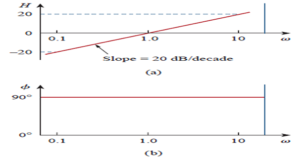
Pole \((j\omega)^{-1}\) at origin:

Bode plots are similar except mag. slope is -20 dB/decade while phase is \(-90^{\circ}\).
For \((j\omega)^{N}\), they are \(20N\) dB/decade and \(90N\) degrees.

Decade : an interval between two frequencies with a ratio of 10; e.g., 10 and 100 Hz. Thus, 20 dB/decade means mag. changes 20 dB whenever the frequency changes tenfold or one decade.

Simple zero \((1+j\omega/z_1)\) :

\[\begin{aligned} \text{Magnitude:}~& 20\log_{10}|1+j\omega/z_1| \\ \text{Phase:}~& \tan^{-1}\omega/z_1 \\ H_{\mathrm{dB}}& =20 \log _{10}\left|1+\frac{j \omega}{z_{1}}\right| \\ \Rightarrow & \omega \rightarrow 0 \quad \quad 20 \log _{10} 1=0 \\ \Rightarrow & \omega \rightarrow \infty \quad 20 \log _{10}\left|1+\frac{\omega}{z_{1}}\right| \end{aligned}\]

Small \(\omega\) mag. approx. to zero (straight line with zero slope)
Large \(\omega\) slope 20 dB/decade
Corner or break frequency: \(\omega = z_1\), two asymptotic lines meet
Approx. and actual plots are close except at \(\omega = z_1\) and deviation is \(20\log_{10}\left|(1+j1)\right|= 20\log_{10}\sqrt{2} = 3~\mathrm{dB}\)

\[\phi = \tan^{-1}\left( \dfrac{\omega}{z_1}\right) = \begin{cases} 0 \quad \omega = 0 \\ 45^{\circ} \quad \omega = z_1 \\ 90^{\circ} \quad \omega \rightarrow \infty \end{cases}\]
Phase
\[\begin{aligned} \phi &= 0 \qquad \omega \leq z_1/10 \\ \phi &= 45^{\circ} \qquad \omega = z_1 \\ \phi &= 90^{\circ} \qquad \omega \geq 10z_1 \end{aligned}\]
straight line approx.

Simple pole \(1/(1+j\omega/p_1)\) :

Plots are similar except at \(\omega = p_1\), magnitude slope is -20 dB/decade and phase slope is \(-45^{\circ}\) per decade

Quadratic pole \(1 /[1+\) \(\left.j 2 \zeta_{2} \omega / \omega_{n}+\left(j \omega / \omega_{n}\right)^{2}\right]\)

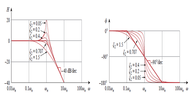
Magnitude : \(-20 \log _{10}\left|1+j 2 \zeta_{2} \omega / \omega_{n}+\left(j \omega / \omega_{n}\right)^{2}\right|\)
Phase \(-\tan ^{-1}\left(2 \zeta_{2} \omega / \omega_{n}\right) /\left(1-\omega^{2} / \omega_{n}^{2}\right)\)

\[\begin{aligned} H_{\mathrm{dB}}&=-20 \log _{10}\left|1+\frac{j 2 \zeta_{2} \omega}{\omega_{n}}+\left(\frac{j \omega}{\omega_{n}}\right)^{2}\right| \Rightarrow 0 \quad \text{as}~ \omega \rightarrow 0\\ H_{\mathrm{dB}}&=-20 \log _{10}\left|1+\frac{j 2 \zeta_{2} \omega}{\omega_{n}}+\left(\frac{j \omega}{\omega_{n}}\right)^{2}\right| \Rightarrow -40 \log _{10} \frac{\omega}{\omega_{n}} \quad \text{as}~ \omega \rightarrow \infty \end{aligned}\]

Amplitude plot consists of two straight asymptotic lines: one with zero slope for \(\omega<\omega_{n}\) and the other with slope \(-40 \mathrm{~dB} /\) decade for \(\omega>\omega_{n}\), with \(\omega_{n}\) as the corner frequency.
Actual plot depends on the damping factor \(\zeta_{2}\) as well as \(\omega_{n}\).
The significant peaking in the neighbourhood of \(\omega_{n}\) should be added to the straight-line approximation if a high level of accuracy is desired.
However, we will use the straight-line approximation for the sake of simplicity.

\[\phi=-\tan ^{-1} \frac{2 \zeta_{2} \omega / \omega_{n}}{1-\omega^{2} / \omega_{n}^{2}}=\left\{\begin{aligned} 0, & ~\omega=0 \\ -90^{\circ}, & ~ \omega=\omega_{n} \\ -180^{\circ}, & ~ \omega \rightarrow \infty \end{aligned}\right.\]

The phase plot is a straight line with a slope of \(-90^{\circ}\) per decade starting at \(\omega_{n} / 10\) and ending at \(10 \omega_{n}\)
Again difference between actual and straight-line plot is due to damping factor.

Notice straight-line approx. for the quadratic pole are the same as those for a double pole, i.e. \(\left(1+j \omega / \omega_{n}\right)^{-2}\) because the double pole equals the quadratic pole \(1 /[1+\) \(\left.j 2 \zeta_{2} \omega / \omega_{n}+\left(j \omega / \omega_{n}\right)^{2}\right]\) when \(\zeta_{2}=1\).
Thus, the quadratic pole can be treated as a double pole as far as straight-line approximation is concerned.
For the quadratic zero \(\left[1+j 2 \zeta_{1} \omega / \omega_{k}+\left(j \omega / \omega_{k}\right)^{2}\right]\), the plots in Fig. are inverted because the magnitude plot has a slope of \(40 \mathrm{~dB} /\) decade while the phase plot has a slope of \(90^{\circ}\) per decade.

Bode straight-line approximations

Problem

\[\begin{aligned} \mathbf{H}(\omega) &=\frac{200 j \omega}{(j \omega+2)(j \omega+10)} \\ \mathbf{H}(\omega)=& \frac{10 j \omega}{(1+j \omega / 2)(1+j \omega / 10)} \qquad \Leftarrow \text{Standard form}\\ =& \frac{10|j \omega|}{|1+j \omega / 2||1+j \omega / 10|} \angle{90^{\circ}-\tan ^{-1} \omega / 2-\tan ^{-1} \omega / 10} \\ H_{\mathrm{dB}}=& 20 \log _{10} 10+20 \log _{10}|j \omega|-20 \log _{10}\left|1+\frac{j \omega}{2}\right| -20 \log _{10}\left|1+\frac{j \omega}{10}\right| \\ \phi=& 90^{\circ}-\tan ^{-1} \frac{\omega}{2}-\tan ^{-1} \frac{\omega}{10} \end{aligned}\]

Construct the bode plots for the given TF

Note: Two corner frequencies at \(\omega = 2, ~10\)

\[\begin{aligned} H_{\mathrm{dB}}=& 20 \log _{10} 10+20 \log _{10}|j \omega|-20 \log _{10}\left|1+\frac{j \omega}{2}\right| -20 \log _{10}\left|1+\frac{j \omega}{10}\right| \\ \phi=& 90^{\circ}-\tan ^{-1} \frac{\omega}{2}-\tan ^{-1} \frac{\omega}{10} \end{aligned}\]