RL Circuit Behavior: Natural Response and Singularity Functions

Concept Demonstration (JoVE)

Demonstrative Video

SECTION 01

Demonstrative Video

SECTION 02

RL Circuit without Source

SECTION 01

The Source-Free RL Circuit

We consider R-L circuits now.
The methods and solutions are very similar to those of RC circuits
The steps involved in solving simple RL or RC circuits containing dc sources:
1. Apply KCL & KVL to write the circuit equation.
2. If the equation contains integrals, differentiate each term in the equation to produce a pure differential equation.
3. Assume a solution of the form \(K_1 + K_2e^{st}\).
4. Substitute the solution into the differential equation to determine the values of \(K_1\) and \(s\). (Alternatively, we can determine \(K_1\) by solving the circuit in steady state )
5. Use the initial conditions to determine the value of \(K_2\).
6. Write the final solution.

SECTION 01

RL Transient Analysis

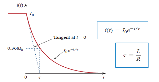
\[\begin{aligned} &i(0)=I_{0} \\ &w(0)=\frac{1}{2} L I_{0}^{2} \\ &v_{L}+v_{R}=0 \\ &L \frac{d i}{d t}+R i=0 \\ &\frac{d i}{d t}+\frac{R}{L} i=0 \\ &\int_{I_{0}}^{i(t)} \frac{d i}{i}=-\int_{0}^{t} \frac{R}{L} d t \end{aligned}\]

\[\left.\ln i\right|_{I_{0}} ^{i(t)}=-\left.\frac{R t}{L}\right|_{0} ^{t} \quad \Rightarrow \quad \ln i(t)-\ln I_{0}=-\frac{R t}{L}+0\]

The natural response of the RL circuit is an exponential decay of the initial current.
\(\tau = L/R\) is time-constant having the unit of seconds

\[\begin{gathered} v_{R}(t)=i R=I_{0} R e^{-t / \tau} \\ p=v_{R} i=I_{0}^{2} R e^{-2 t / \tau} \\ w_{R}(t)=\int_{0}^{t} p d t=\int_{0}^{t} I_{0}^{2} R e^{-2 t / \tau} d t=-\left.\frac{1}{2} \tau I_{0}^{2} R e^{-2 t / \tau}\right|_{0} ^{t} \\ w_{R}(t)=\frac{1}{2} L I_{0}^{2}\left(1-e^{-2 t / \tau}\right) \end{gathered}\]

Note that as \(t \rightarrow \infty, w_{R}(\infty) \rightarrow \frac{1}{2} L I_{0}^{2}\), which is the same as \(w_{L}(0)\), the initial energy stored in the inductor
Again, the energy initially stored in the inductor is eventually dissipated in the resistor.

SECTION 01

Problem solving steps

Determine \(i(0)=I_0\) through the inductor
Determine time constant \(\tau\) of the circuit
Inductor current \(i_L(t)=i(t)=i(0)e^{-t/\tau}\)
Once \(i_L\) is determined, other variables \(v_L\), \(v_R\), and \(i_R\) can be obtained
Note: \(R\) is \(R_{TH}\) at the inductor terminals.

SECTION 01

Solved Problem

Assuming \(i(0)=10\) A, calculate \(i(t)\) and \(i_x(t)\)

\[\begin{aligned} &2\left(i_{1}-i_{2}\right)+1=0 \quad \Rightarrow i_{1}-i_{2}=-\frac{1}{2} \\ &6 i_{2}-2 i_{1}-3 i_{1}=0 \quad \Rightarrow \quad i_{2}=\frac{5}{6} i_{1} \\ &i_{1}=-3 \mathrm{~A}, \quad i_{o}=-i_{1}=3 \mathrm{~A} \end{aligned}\]

\[\begin{aligned} &R_{\mathrm{eq}}=R_{\mathrm{Th}}=\frac{v_{o}}{i_{o}}=\frac{1}{3} \Omega \\ &\tau=\frac{L}{R_{\mathrm{eq}}}=\frac{\frac{1}{2}}{\frac{1}{3}}=\frac{3}{2} \mathrm{~s} \\ &i(t)=i(0) e^{-t / \tau}=10 e^{-(2 / 3) t} \mathrm{~A} \end{aligned}\]

SECTION 01

Singularity Functions

A basic understanding of singularity functions will help us make sense of the response of first-order circuits to a sudden application of an independent dc voltage or current source.
Singularity functions (also called switching functions) are very useful in circuit analysis.
They serve as good approximations to the switching signals that arise in circuits with switching operations.
Singularity functions are functions that either are discontinuous or have discontinuous derivatives.
The three most widely used singularity functions in circuit analysis are the unit step, the unit impulse, and the unit ramp functions

SECTION 01

Unit Step-function

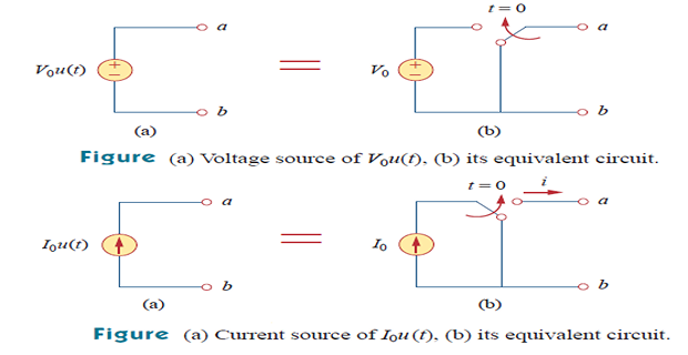
\[\begin{gathered} u(t)= \begin{cases}0, & t<0 \\ 1, & t>0\end{cases} \\ u\left(t-t_{0}\right)= \begin{cases}0, & t<t_{0} \\ 1, & t>t_{0}\end{cases} \\ u\left(t+t_{0}\right)= \begin{cases}0, & t<-t_{0} \\ 1, & t>-t_{0}\end{cases} \end{gathered}\]

\[v(t)= \begin{cases}0, & t<t_{0} \\ V_{0}, & t>t_{0}\end{cases} \Rightarrow~v(t)=V_{0} u\left(t-t_{0}\right)\]
We use the step function to represent an abrupt change in voltage or current, like the changes that occur in the circuits of control systems and digital computers. For example, the voltage

SECTION 01

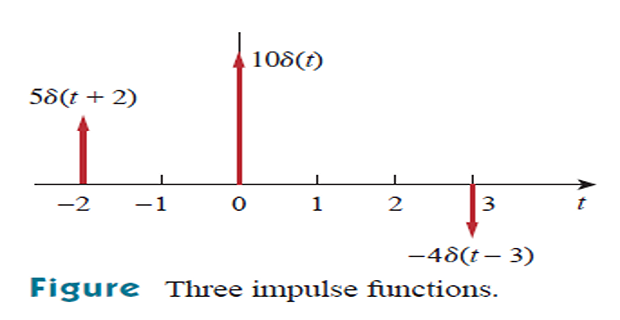
Unit Impulse function

The derivative of the unit step function \(u(t)\) is the unit impulse function \(\delta(t)\)
The unit impulse function \(\delta(t)\) is zero everywhere except at \(t=0\), where it is undefined.

\[\delta(t)=\frac{d}{d t} u(t)= \begin{cases}0, & t<0 \\ \text { Undefined, } & t=0 \\ 0, & t>0\end{cases}\]

Impulsive currents and voltages occur in electric circuits as a result of switching operations or impulsive sources.
Although the unit impulse function is not physically realizable (just like ideal sources, ideal resistors, etc.), it is a very useful mathematical tool.
The unit impulse may be regarded as an applied or resulting shock.
It may be visualized as a very short duration pulse of unit area.
\[\int_{0^{-}}^{0^{+}} \delta(t) d t=1\]
This may be expressed mathematically as

The unit area is known as the strength of the impulse function.
When an impulse function has a strength other than unity, the area of the impulse is equal to its strength

SECTION 01

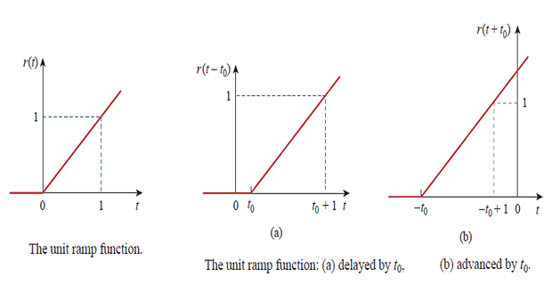
Unit-Ramp Function

Integrating the unit step-function \(u(t)\) is the ramp-function \(r(t)\)

\[\begin{aligned} &r(t)=\int_{-\infty}^{t} u(t) d t=t u(t) \\ &r(t)= \begin{cases}0, & t \leq 0 \\ t, & t \geq 0\end{cases} \\ &r\left(t-t_{0}\right)= \begin{cases}0, & t \leq t_{0} \\ t-t_{0}, & t \geq t_{0}\end{cases} \\ &r\left(t+t_{0}\right)= \begin{cases}0, & t \leq-t_{0} \\ t+t_{0}, & t \geq-t_{0}\end{cases} \end{aligned}\]