- Distinguish a one-port from a two-port network and state the port condition.
- Determine the impedance (\(z\)) parameters by open-circuit measurements.
- Determine the admittance (\(y\)) parameters by short-circuit measurements.
- Determine the hybrid (\(h\)) parameters and explain why they suit transistors.
- Determine the transmission (\(ABCD\)) parameters and explain why they suit cascades.
- Convert between any two parameter sets.
- Test a network for reciprocity and symmetry.
- Combine two-ports connected in series, parallel and cascade.
- Apply \(h\) parameters to compute the gains and impedances of a transistor amplifier.
Introduction
A port is a pair of terminals through which current may enter and leave a network. The defining requirement — the port condition — is that the current entering one terminal must equal the current leaving the other.
A one-port network has a single such pair. Chapter 4's Thévenin equivalent was exactly this: a whole network, however elaborate, reduced to what a single pair of terminals sees. Series and parallel combinations of resistors and capacitors are one-ports.
A two-port network has two pairs — an input port and an output port. Amplifiers, attenuators, filters and transformers are all two-ports, and so are transistors, transmission lines and coupled coils.
The idea driving this chapter is worth stating plainly. A two-port may contain a single resistor or ten thousand transistors; from outside it makes no difference. All that can be observed is the relationship among four quantities — \(\mathbf{V}_{1}\), \(\mathbf{I}_{1}\), \(\mathbf{V}_{2}\), \(\mathbf{I}_{2}\) — and for a linear network that relationship is captured by just four parameters.
This is enormously useful. A manufacturer can characterise a device without disclosing its design; a designer can predict a cascade's behaviour without analysing every stage; and measurement replaces analysis entirely where the internals are unknown or inaccessible.
Two conventions apply throughout: both currents are taken as entering the network at the upper terminal of each port, and no independent sources are present inside — dependent sources are allowed, and are what make amplifiers possible.
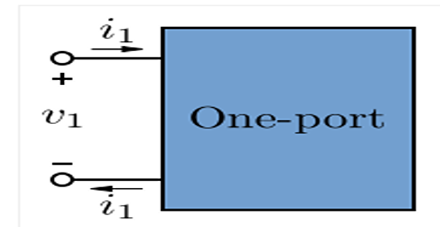
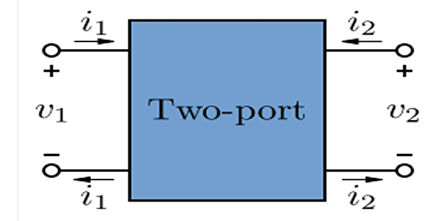
With four terminal quantities, any two may be chosen as independent and the other two expressed in terms of them. That choice gives six parameter sets, of which four are in common use.
| Set | Expresses | In terms of | Typical use |
|---|---|---|---|
| \(z\) impedance | \(\mathbf{V}_{1}, \mathbf{V}_{2}\) | \(\mathbf{I}_{1}, \mathbf{I}_{2}\) | series connections, filters |
| \(y\) admittance | \(\mathbf{I}_{1}, \mathbf{I}_{2}\) | \(\mathbf{V}_{1}, \mathbf{V}_{2}\) | parallel connections |
| \(h\) hybrid | \(\mathbf{V}_{1}, \mathbf{I}_{2}\) | \(\mathbf{I}_{1}, \mathbf{V}_{2}\) | transistors |
| \(ABCD\) transmission | \(\mathbf{V}_{1}, \mathbf{I}_{1}\) | \(\mathbf{V}_{2}, \mathbf{I}_{2}\) | cascades, transmission lines |
The remaining two — the inverse hybrid \(g\) and inverse transmission \(abcd\) — are simply the matrix inverses of the last two and are used only occasionally. No set is more correct than another; each is chosen because it makes some particular calculation easy, and Section 19.6 converts freely between them.
Impedance Parameters
Taking the currents as independent gives
Each parameter is isolated by setting one current to zero — that is, by open-circuiting the corresponding port. Hence the alternative name open-circuit parameters.
| Parameter | Name | Condition |
|---|---|---|
| \(z_{11}\) | open-circuit input impedance | output open |
| \(z_{12}\) | open-circuit reverse transfer impedance | input open |
| \(z_{21}\) | open-circuit forward transfer impedance | output open |
| \(z_{22}\) | open-circuit output impedance | input open |
All four have units of ohms. Note the index convention: the first subscript identifies where the voltage is measured, the second where the current is applied.
A caution. The \(z\) parameters do not exist for every network. A network whose \(z\) matrix is singular has no \(y\) parameters, and vice versa — an ideal transformer, for instance, has neither. This is one reason several parameter sets are needed.
Problem. A T network has a 20 \(\Omega\) series arm at the input, a 30 \(\Omega\) series arm at the output, and a 40 \(\Omega\) shunt arm between them. Find its \(z\) parameters.
Solution. Take each parameter in turn.
\(z_{11}\): open-circuit port 2, so no current flows in the 30 \(\Omega\) arm and it contributes nothing. The input sees 20 \(\Omega\) in series with 40 \(\Omega\):
\(z_{21}\): with port 2 open, \(\mathbf{V}_{2}\) is the voltage across the 40 \(\Omega\) shunt — again because no current flows through the 30 \(\Omega\) and there is no drop across it:
\(z_{22}\) and \(z_{12}\): by the mirror argument with port 1 open,
Two observations. The shunt element appears in every parameter, since it is common to both loops — this is the general pattern for a T network, whose parameters are \(z_{11} = Z_{a}+Z_{c}\), \(z_{12} = z_{21} = Z_{c}\), \(z_{22} = Z_{b}+Z_{c}\). And \(z_{12} = z_{21}\), which makes the network reciprocal — a property of any network built only from R, L, C and mutual inductance, as Section 19.7 explains.
The determinant \(\Delta_{z} = 2600\) will be needed repeatedly; this same network runs through Examples 19.3 to 19.6.
Admittance Parameters
Taking the voltages as independent gives the dual set:
Each parameter is found by setting a voltage to zero — by short-circuiting a port — hence short-circuit parameters:
All four are in siemens. The \(y\) matrix is the inverse of the \(z\) matrix — not the reciprocal of each element, a distinction Section 19.6 makes precise.
Where \(z\) parameters suit a T network, \(y\) parameters suit a Pi network, whose parameters can be written down by inspection:
where \(Y_{2}\) is the series branch and \(Y_{1}\), \(Y_{3}\) the two shunts. Note the minus sign on the transfer terms: it arises because a positive \(\mathbf{V}_{2}\) drives current out of port 1 through the shared branch. Off-diagonal \(y\) parameters are negative for any passive network.
Problem. A Pi network has a 5 \(\Omega\) shunt at the input, a 10 \(\Omega\) series branch, and a 20 \(\Omega\) shunt at the output. Find its \(y\) parameters.
Solution. Convert each resistance to an admittance: \(Y_{1} = 0.2\), \(Y_{2} = 0.1\), \(Y_{3} = 0.05~\mathrm{S}\).
\(y_{11}\): short-circuit port 2. The 20 \(\Omega\) shunt is then shorted out entirely, and the input sees the 5 \(\Omega\) in parallel with the 10 \(\Omega\):
\(y_{21}\): with port 2 shorted, all the current through the 10 \(\Omega\) flows out of port 2 — out, so with the entering-current convention it is negative:
\(y_{22}\) and \(y_{12}\): by symmetry of argument,
Again \(y_{12} = y_{21}\), confirming reciprocity. The Pi network is the exact dual of the T: shunt admittances play the role that series impedances played before.
Hybrid Parameters
Neither \(z\) nor \(y\) parameters suit a transistor. A transistor's input behaves like a low impedance and its output like a high one, so open-circuiting the input or short-circuiting the output is awkward in practice. The hybrid parameters mix the two descriptions to match:
The four have different units — which is exactly why they are called hybrid:
| Parameter | Name | Units | Transistor symbol |
|---|---|---|---|
| \(h_{11}\) | short-circuit input impedance | ohms | \(h_{ie}\) |
| \(h_{12}\) | open-circuit reverse voltage gain | dimensionless | \(h_{re}\) |
| \(h_{21}\) | short-circuit forward current gain | dimensionless | \(h_{fe}\) |
| \(h_{22}\) | open-circuit output admittance | siemens | \(h_{oe}\) |
The subscript letters denote input, reverse, forward, output, and the trailing \(e\) denotes the common-emitter configuration. \(h_{fe}\) is the current gain \(\beta\) familiar from transistor work — its appearance here as a two-port parameter is the reason the whole scheme is standard in electronics.
The inverse hybrid or \(g\) parameters swap the roles, expressing \(\mathbf{I}_{1}\) and \(\mathbf{V}_{2}\) in terms of \(\mathbf{V}_{1}\) and \(\mathbf{I}_{2}\). The \(g\) matrix is the inverse of the \(h\) matrix.
Problem. Find the \(h\) parameters of the T network of Example 19.1, for which \(\left[z\right] = \begin{bmatrix}60&40\\40&70\end{bmatrix}\) and \(\Delta_{z} = 2600\).
Solution. Using the conversion formulas of Section 19.6:
Check the units: ohms, dimensionless, dimensionless, siemens — as required for a hybrid set.
Check reciprocity: for a reciprocal network the \(h\) condition is \(h_{12} = -h_{21}\), and indeed \(0.5714 = -(-0.5714)\) \(\checkmark\). Note that this differs from the \(z\) and \(y\) conditions — each parameter set expresses reciprocity differently, and confusing them is a common error.
A negative \(h_{21}\) means the output current flows opposite to the reference direction, which is normal for a passive network — it has no gain and cannot deliver current outward. A transistor's \(h_{fe}\) of \(+50\) or more is the mark of an active device.
Transmission Parameters
The transmission or ABCD parameters express the input quantities in terms of the output ones — the natural direction for a signal travelling through a chain of networks:
Note the minus signs. They arise because the convention here takes \(\mathbf{I}_{2}\) as leaving the network, matching the physical picture of current flowing onward into the next stage. This is the one place in the chapter where the entering-current convention is set aside, and it must be remembered when converting.
| Parameter | Name | Units |
|---|---|---|
| \(A\) | open-circuit voltage ratio | dimensionless |
| \(B\) | negative short-circuit transfer impedance | ohms |
| \(C\) | open-circuit transfer admittance | siemens |
| \(D\) | negative short-circuit current ratio | dimensionless |
These parameters are indispensable for transmission lines and for any cascade, because — as Section 19.8 shows — cascaded networks multiply their \(ABCD\) matrices. No other parameter set has that property.
Problem. Find the transmission parameters of the same T network, and verify the reciprocity condition.
Solution. From the conversion formulas:
The reciprocity check for transmission parameters is that the determinant equals unity:
This is the most elegant of all the reciprocity conditions, and the most useful in practice: any arithmetic slip in computing \(A\), \(B\), \(C\) or \(D\) will almost certainly break it. Always check.
Note also that \(A \neq D\) here. Equality would indicate a symmetric network, and this one is not — its two series arms differ (20 \(\Omega\) against 30 \(\Omega\)). Making them equal would give \(z_{11} = z_{22}\) and hence \(A = D\).
Relationships Between Parameters
Since all four sets describe the same network, any one determines the rest. The derivation is straightforward algebra: solve one pair of equations for the desired variables and read off the coefficients.
The \(z\)-to-\(y\) relationship is the cleanest, because the two matrices are simply inverses:
with \(\Delta_{z} = z_{11}z_{22}-z_{12}z_{21}\). It follows immediately that \(\Delta_{y} = 1/\Delta_{z}\).
Note carefully: \(y_{11} \neq 1/z_{11}\). The matrices are inverses, not the individual elements. This is the single most common error in the whole chapter.
| To find | From \(z\) | From \(y\) | From \(h\) |
|---|---|---|---|
| \(z_{11}\) | — | \(y_{22}/\Delta_{y}\) | \(\Delta_{h}/h_{22}\) |
| \(z_{12}\) | — | \(-y_{12}/\Delta_{y}\) | \(h_{12}/h_{22}\) |
| \(z_{21}\) | — | \(-y_{21}/\Delta_{y}\) | \(-h_{21}/h_{22}\) |
| \(z_{22}\) | — | \(y_{11}/\Delta_{y}\) | \(1/h_{22}\) |
| \(h_{11}\) | \(\Delta_{z}/z_{22}\) | \(1/y_{11}\) | — |
| \(h_{12}\) | \(z_{12}/z_{22}\) | \(-y_{12}/y_{11}\) | — |
| \(h_{21}\) | \(-z_{21}/z_{22}\) | \(y_{21}/y_{11}\) | — |
| \(h_{22}\) | \(1/z_{22}\) | \(\Delta_{y}/y_{11}\) | — |
| \(A\) | \(z_{11}/z_{21}\) | \(-y_{22}/y_{21}\) | \(-\Delta_{h}/h_{21}\) |
| \(B\) | \(\Delta_{z}/z_{21}\) | \(-1/y_{21}\) | \(-h_{11}/h_{21}\) |
| \(C\) | \(1/z_{21}\) | \(-\Delta_{y}/y_{21}\) | \(-h_{22}/h_{21}\) |
| \(D\) | \(z_{22}/z_{21}\) | \(-y_{11}/y_{21}\) | \(-1/h_{21}\) |
There is no need to memorise this table. Two things are worth remembering instead: \(\left[y\right] = \left[z\right]^{-1}\), and that any conversion can be re-derived in a minute by solving the defining equations. The determinants \(\Delta_{z}\), \(\Delta_{y}\) and \(\Delta_{h}\) appear throughout, so compute them first.
Problem. Find the \(y\) parameters of the T network of Example 19.1, and verify the determinant relationship.
Solution. With \(\Delta_{z} = 2600\):
Verification. The determinant should be the reciprocal of \(\Delta_{z}\):
Note that \(y_{11} = 0.02692\) while \(1/z_{11} = 1/60 = 0.01667\) — quite different numbers. The elements are not reciprocals of one another, only the matrices are inverses. And observe that the off-diagonal \(y\) terms have come out negative, as predicted for a passive network in Section 19.3.
Reciprocity and Symmetry
Two structural properties reduce the four parameters to three or two, and both have simple physical meanings.
Reciprocity. A network is reciprocal if interchanging an ideal voltage source and an ideal ammeter between the two ports leaves the ammeter reading unchanged. Every network built solely from resistors, inductors, capacitors and mutual inductance is reciprocal; only networks containing dependent sources — that is, active devices — can fail to be.
The condition takes a different algebraic form in each parameter set, which is a persistent source of confusion:
| Set | Reciprocity condition | Symmetry condition |
|---|---|---|
| \(z\) | \(z_{12} = z_{21}\) | \(z_{11} = z_{22}\) |
| \(y\) | \(y_{12} = y_{21}\) | \(y_{11} = y_{22}\) |
| \(h\) | \(h_{12} = -h_{21}\) | \(\Delta_{h} = 1\) |
| \(ABCD\) | \(AD-BC = 1\) | \(A = D\) |
Symmetry. A network is symmetric if its two ports may be interchanged without any observable difference — electrically, the network looks the same from either end. A symmetric network is necessarily reciprocal, but the converse does not hold: the T network of Example 19.1 is reciprocal (\(z_{12} = z_{21} = 40\)) yet not symmetric (\(z_{11} = 60 \neq 70 = z_{22}\)), because its series arms differ.
A symmetric network has only two independent parameters instead of four, and its \(ABCD\) matrix satisfies both \(A = D\) and \(AD-BC = 1\). Symmetric sections are the building blocks of classical filter design, precisely because identical sections can be cascaded without impedance mismatches at the joins.
Interconnection of Two-Ports
The practical power of the two-port description appears when networks are combined. Each connection type has a parameter set for which the combination rule is trivial — and that is why several sets exist.
Series connection. Both inputs are in series and both outputs are in series, so the currents are shared and the voltages add. Since \(z\) parameters give voltage in terms of current, the matrices simply add:
Parallel connection. The voltages are shared and the currents add, so by the dual argument:
Cascade connection. The output of the first network becomes the input of the second, which is precisely the relation \(ABCD\) parameters express. The matrices multiply:
The order matters, since matrix multiplication does not commute. \(\left[T_{1}\right]\) is written first because the signal encounters \(N_{1}\) first. Reversing the order describes a physically different circuit.
A caution on series and parallel connections. The addition rules assume the port condition still holds after connection — that the current entering each port's upper terminal still equals that leaving its lower one. Interconnecting two-ports can violate this, in which case the rules fail. The Brune test checks for it, and cascade connection is free of the difficulty entirely, which is one more reason the \(ABCD\) set is the most used in practice.
Problem. Two identical T networks, each with the parameters of Example 19.4, are connected in cascade. Find the overall transmission parameters, and verify reciprocity.
Solution. Multiply the matrices:
Element by element:
Verification.
The cascade is still reciprocal, as it must be — a cascade of passive networks cannot become active. More generally, since the determinant of a product equals the product of the determinants, any cascade of reciprocal networks is reciprocal, each factor contributing a determinant of 1.
Note how much has changed: \(A\) has risen from 1.5 to 3.875, meaning the input voltage must now be nearly four times the output. Two attenuating sections attenuate more than one — obvious in principle, but here quantified by a single matrix multiplication rather than a fresh circuit analysis.
Practical Engineering Applications
The dominant application of two-port theory is the small-signal analysis of transistor amplifiers. A manufacturer publishes the four \(h\) parameters, and every important amplifier property follows from them without any knowledge of the device's internal physics.
With a load \(R_{L}\) connected at the output, the standard results are
where \(\Delta_{h} = h_{ie}h_{oe}-h_{re}h_{fe}\). The negative voltage gain signals the phase inversion characteristic of a common-emitter stage.
Problem. A transistor has \(h_{ie} = 1.1~\mathrm{k}\Omega\), \(h_{re} = 2.5\times10^{-4}\), \(h_{fe} = 50\) and \(h_{oe} = 25~\mu\mathrm{S}\). With \(R_{L} = 1~\mathrm{k}\Omega\), find the voltage gain, current gain, power gain and input impedance.
Solution. First the determinant:
Voltage gain:
Current gain:
Power gain is the product of the two magnitudes:
Input impedance:
Reading the results. The stage inverts and amplifies by about 45 in voltage and 49 in current, giving a power gain over 2000 — or 33.4 dB by the convention of Section 14.3. The input impedance is barely below \(h_{ie}\), because \(h_{re}\) is very small and the reverse feedback it represents is nearly negligible. Setting \(h_{re} = 0\) would give \(Z_{\text{in}} = 1100~\Omega\), an error of about 1 % — which is why simplified transistor models routinely drop that term.
Note that \(h_{fe} = +50\) is positive, unlike the \(h_{21} = -0.5714\) of the passive network in Example 19.3. That sign difference is the mathematical signature of an active device.
A transmission line is the two-port par excellence. Its \(ABCD\) parameters are \(A = D = \cosh\gamma\ell\), \(B = Z_{0}\sinh\gamma\ell\) and \(C = \sinh\gamma\ell/Z_{0}\), where \(\gamma\) is the propagation constant and \(Z_{0}\) the characteristic impedance. Note that \(A = D\), as symmetry requires, and that \(AD-BC = \cosh^{2}-\sinh^{2} = 1\), as reciprocity requires.
Because lines in series simply multiply their matrices, a route composed of several line sections, transformers and compensating elements is analysed by multiplying a chain of two-by-two matrices — the standard method in power system analysis.
Ladder networks — alternating series and shunt elements — are handled the same way. A series impedance \(Z\) has the matrix \(\begin{bmatrix}1&Z\\0&1\end{bmatrix}\) and a shunt admittance \(Y\) has \(\begin{bmatrix}1&0\\Y&1\end{bmatrix}\), so any ladder is the product of these two building blocks in the appropriate order. The multi-section filters of Chapter 14 are designed exactly this way.
Two-port parameters can be measured on a network whose internals are unknown or inaccessible — a sealed module, an integrated circuit, a length of cable already installed. Four measurements suffice to characterise it completely for all subsequent design work.
At radio and microwave frequencies, open and short circuits are difficult to realise accurately, so the scattering or \(S\) parameters are used instead. They relate incident and reflected waves rather than voltages and currents, and are measured with matched terminations rather than opens and shorts. The underlying idea is identical to this chapter's, and the conversions between \(S\) and \(z\) parameters are standard.
Summary and Key Formulas
A port is a terminal pair satisfying the port condition; a two-port is fully described by four parameters, whatever it contains.
\(z\) parameters are found by open-circuit tests, \(y\) parameters by short-circuit tests.
\(h\) parameters mix the two and suit transistors, where \(h_{fe}\) is the familiar current gain.
\(ABCD\) parameters express input in terms of output, with \(\mathbf{I}_{2}\) taken as leaving the network.
\(\left[y\right] = \left[z\right]^{-1}\) — the matrices are inverses, not the individual elements.
Reciprocity holds for any network of R, L, C and mutual inductance, and is expressed differently in each parameter set.
Symmetry means the ports may be interchanged; it implies reciprocity but not conversely.
Series connections add \(z\), parallel connections add \(y\), cascades multiply \(T\) — and cascade order matters.
Transistor gains and impedances follow from the four \(h\) parameters alone.
The condition \(AD-BC = 1\) is the most convenient arithmetic check in the whole chapter.
| Result | Formula | Notes |
|---|---|---|
| \(z\) parameters | \(\mathbf{V} = \left[z\right]\mathbf{I}\) | open-circuit tests |
| \(y\) parameters | \(\mathbf{I} = \left[y\right]\mathbf{V}\) | short-circuit tests |
| \(h\) parameters | \(\mathbf{V}_{1} = h_{11}\mathbf{I}_{1}+h_{12}\mathbf{V}_{2}\), \(\mathbf{I}_{2} = h_{21}\mathbf{I}_{1}+h_{22}\mathbf{V}_{2}\) | mixed units |
| \(ABCD\) | \(\mathbf{V}_{1} = A\mathbf{V}_{2}-B\mathbf{I}_{2}\), \(\mathbf{I}_{1} = C\mathbf{V}_{2}-D\mathbf{I}_{2}\) | note the signs |
| T network | \(z_{11} = Z_{a}+Z_{c}\), \(z_{12} = z_{21} = Z_{c}\), \(z_{22} = Z_{b}+Z_{c}\) | by inspection |
| Pi network | \(y_{11} = Y_{1}+Y_{2}\), \(y_{12} = y_{21} = -Y_{2}\), \(y_{22} = Y_{2}+Y_{3}\) | note the minus |
| \(z \to y\) | \(\left[y\right] = \left[z\right]^{-1}\), \(\Delta_{y} = 1/\Delta_{z}\) | matrices, not elements |
| \(z \to h\) | \(h_{11} = \Delta_{z}/z_{22}\), \(h_{22} = 1/z_{22}\) | and \(h_{12} = z_{12}/z_{22}\) |
| \(z \to ABCD\) | \(A = z_{11}/z_{21}\), \(B = \Delta_{z}/z_{21}\), \(C = 1/z_{21}\), \(D = z_{22}/z_{21}\) | |
| Reciprocity | \(z_{12}=z_{21}\); \(y_{12}=y_{21}\); \(h_{12}=-h_{21}\); \(AD-BC=1\) | differs by set |
| Symmetry | \(z_{11}=z_{22}\); \(y_{11}=y_{22}\); \(\Delta_{h}=1\); \(A=D\) | implies reciprocity |
| Series connection | \(\left[z\right] = \left[z_{1}\right]+\left[z_{2}\right]\) | matrices add |
| Parallel connection | \(\left[y\right] = \left[y_{1}\right]+\left[y_{2}\right]\) | matrices add |
| Cascade | \(\left[T\right] = \left[T_{1}\right]\left[T_{2}\right]\) | order matters |
| Series element | \(\begin{bmatrix}1&Z\\0&1\end{bmatrix}\) | ladder block |
| Shunt element | \(\begin{bmatrix}1&0\\Y&1\end{bmatrix}\) | ladder block |
| Transistor voltage gain | \(A_{v} = \dfrac{-h_{fe}R_{L}}{h_{ie}+\Delta_{h}R_{L}}\) | negative: inverting |
| Transistor current gain | \(A_{i} = \dfrac{h_{fe}}{1+h_{oe}R_{L}}\) | |
| Transistor input impedance | \(Z_{\text{in}} = h_{ie}-\dfrac{h_{re}h_{fe}R_{L}}{1+h_{oe}R_{L}}\) |
Common Mistakes
Taking \(y_{11} = 1/z_{11}\). The matrices are inverses; the elements are not reciprocals. In Example 19.5 the two differ by a factor of 1.6.
Getting the current convention wrong. Both currents enter the network for \(z\), \(y\) and \(h\) parameters — but \(\mathbf{I}_{2}\) is taken as leaving for \(ABCD\), which is where the minus signs come from.
Using the wrong reciprocity condition. It is \(z_{12} = z_{21}\) but \(h_{12} = -h_{21}\) and \(AD-BC = 1\). Applying one set's condition to another is a frequent error.
Confusing reciprocity with symmetry. Every symmetric network is reciprocal; most reciprocal networks are not symmetric. Example 19.1's T network is the case in point.
Reversing the cascade order. \(\left[T_{1}\right]\left[T_{2}\right]\) and \(\left[T_{2}\right]\left[T_{1}\right]\) describe different circuits.
Adding \(z\) matrices for a parallel connection. Series adds \(z\), parallel adds \(y\). Only cascade uses \(T\).
Forgetting the minus sign in a Pi network's \(y_{12}\). Off-diagonal \(y\) parameters are negative for passive networks.
Assuming every network has every parameter set. An ideal transformer has neither \(z\) nor \(y\) parameters, though it has \(ABCD\) parameters.
Including independent sources inside the two-port. The definitions assume none; dependent sources are permitted and are what make active two-ports possible.
Skipping the \(AD-BC = 1\) check. It costs one line and catches nearly every arithmetic slip.
Chapter Review
Work these before opening the answers. Verify reciprocity wherever it applies.
P19.1 Find the \(z\) parameters of a T network with series arms of 10 \(\Omega\) and 10 \(\Omega\) and a shunt of 25 \(\Omega\). Is it symmetric?
Show answer
Since \(z_{11} = z_{22}\) the network is symmetric, and being made of resistors it is also reciprocal. Only two parameters are independent.\[z_{11} = 10+25 = 35~\Omega, \quad z_{12} = z_{21} = 25~\Omega, \quad z_{22} = 10+25 = 35~\Omega\]P19.2 A two-port has \(\left[z\right] = \begin{bmatrix}10&6\\6&8\end{bmatrix}~\Omega\). Find its \(y\) parameters.
Show answer
\[\Delta_{z} = 80-36 = 44\]Check: \(\Delta_{y} = (0.1818)(0.2273)-(0.1364)^{2} = 0.02273 = 1/44\) \(\checkmark\)\[y_{11} = \frac{8}{44} = 0.1818, \quad y_{12} = y_{21} = \frac{-6}{44} = -0.1364, \quad y_{22} = \frac{10}{44} = 0.2273~\mathrm{S}\]P19.3 Find the \(h\) parameters of the network in P19.2.
Show answer
\[h_{11} = \frac{\Delta_{z}}{z_{22}} = \frac{44}{8} = 5.500~\Omega, \qquad h_{12} = \frac{6}{8} = 0.7500\]Reciprocity: \(h_{12} = -h_{21}\) \(\checkmark\)\[h_{21} = -\frac{6}{8} = -0.7500, \qquad h_{22} = \frac{1}{8} = 0.1250~\mathrm{S}\]P19.4 Find the \(ABCD\) parameters of the network in P19.2 and verify reciprocity.
Show answer
\[A = \frac{10}{6} = 1.667, \quad B = \frac{44}{6} = 7.333~\Omega, \quad C = \frac{1}{6} = 0.1667~\mathrm{S}, \quad D = \frac{8}{6} = 1.333\]\[AD-BC = \left(1.667\right)\left(1.333\right)-\left(7.333\right)\left(0.1667\right) = 2.222-1.222 = 1.000 \;\checkmark\]P19.5 Write the \(ABCD\) matrix of a single series impedance \(Z\), and of a single shunt admittance \(Y\).
Show answer
Both have determinant 1, so both are reciprocal, as any passive element must be.\[\text{Series } Z: \begin{bmatrix}1&Z\\0&1\end{bmatrix}, \qquad \text{Shunt } Y: \begin{bmatrix}1&0\\Y&1\end{bmatrix}\]P19.6 Use P19.5 to find the \(ABCD\) matrix of an L-section: a 4 \(\Omega\) series resistor followed by a 0.5 S shunt.
Show answer
Check: \(AD-BC = 3-2 = 1\) \(\checkmark\)\[\left[T\right] = \begin{bmatrix}1&4\\0&1\end{bmatrix}\begin{bmatrix}1&0\\0.5&1\end{bmatrix} = \begin{bmatrix}1+2&4\\0.5&1\end{bmatrix} = \begin{bmatrix}3&4\\0.5&1\end{bmatrix}\]P19.7 Two two-ports with \(\left[z_{1}\right] = \begin{bmatrix}4&2\\2&5\end{bmatrix}\) and \(\left[z_{2}\right] = \begin{bmatrix}6&3\\3&7\end{bmatrix}\) are connected in series. Find the overall \(z\) matrix.
Show answer
Still reciprocal, since \(z_{12} = z_{21}\) for both components and addition preserves it.\[\left[z\right] = \begin{bmatrix}10&5\\5&12\end{bmatrix}~\Omega\]P19.8 A transistor has \(h_{ie} = 2~\mathrm{k}\Omega\), \(h_{re} = 0\), \(h_{fe} = 100\), \(h_{oe} = 20~\mu\mathrm{S}\), with \(R_{L} = 2~\mathrm{k}\Omega\). Find \(A_{v}\), \(A_{i}\) and \(Z_{\text{in}}\).
Show answer
With \(h_{re} = 0\), \(\Delta_{h} = h_{ie}h_{oe} = (2000)(20\times10^{-6}) = 0.04\).\[A_{v} = \frac{-\left(100\right)\left(2000\right)}{2000+\left(0.04\right)\left(2000\right)} = \frac{-200\,000}{2080} = -96.15\]With no reverse feedback the input impedance is exactly \(h_{ie}\).\[A_{i} = \frac{100}{1+0.04} = 96.15, \qquad Z_{\text{in}} = h_{ie} = 2000~\Omega\]P19.9 A network has \(\left[h\right]\) with \(h_{12} = 0.4\) and \(h_{21} = 0.4\). Is it reciprocal? What does this imply?
Show answer
The reciprocity condition for \(h\) parameters is \(h_{12} = -h_{21}\). Here \(0.4 \neq -0.4\), so the network is not reciprocal. It must therefore contain a dependent source — it is an active network, and cannot be built from R, L, C and mutual inductance alone.P19.10 Explain why the \(ABCD\) parameters of a cascade of \(n\) reciprocal networks always satisfy \(AD-BC = 1\).
Show answer
The overall matrix is the product \(\left[T_{1}\right]\left[T_{2}\right]\cdots\left[T_{n}\right]\), and the determinant of a product equals the product of the determinants. Each factor is reciprocal and so has determinant 1, giving \(1\times1\times\cdots\times1 = 1\). Physically: cascading passive networks cannot create an active one.
MCQ 1. The \(z\) parameters are determined by:
(a) short-circuit tests (b) open-circuit tests (c) matched loads (d) DC measurementsShow answer
(b) open-circuit tests, since each is found by setting a current to zero.MCQ 2. The \(y\) matrix relates to the \(z\) matrix by:
(a) element-by-element reciprocals (b) matrix inversion (c) transposition (d) they are unrelatedShow answer
(b) inversion. Option (a) is the classic error.MCQ 3. The parameter \(h_{21}\) of a transistor is usually written:
(a) \(h_{ie}\) (b) \(h_{re}\) (c) \(h_{fe}\) (d) \(h_{oe}\)Show answer
(c) \(h_{fe}\) — the forward current gain, or \(\beta\).MCQ 4. Which parameter set has elements with different units?
(a) \(z\) (b) \(y\) (c) \(h\) (d) noneShow answer
(c) \(h\) — ohms, dimensionless, dimensionless and siemens. Hence "hybrid". (The \(ABCD\) set is also mixed.)MCQ 5. For a reciprocal network the transmission parameters satisfy:
(a) \(A = D\) (b) \(AD-BC = 1\) (c) \(B = C\) (d) \(A = 1\)Show answer
(b). Option (a) is the symmetry condition.MCQ 6. Two two-ports in parallel combine by:
(a) adding \(z\) matrices (b) adding \(y\) matrices (c) multiplying \(T\) matrices (d) adding \(h\) matricesShow answer
(b). Voltages are shared and currents add, which is what \(y\) parameters express.MCQ 7. Cascaded two-ports combine by:
(a) adding \(z\) (b) adding \(y\) (c) multiplying \(ABCD\) matrices (d) averagingShow answer
(c), in the order the signal encounters them.MCQ 8. A network of resistors, inductors and capacitors is:
(a) always symmetric (b) always reciprocal (c) never reciprocal (d) always activeShow answer
(b) always reciprocal. Symmetry is an additional, separate condition.MCQ 9. A symmetric two-port has how many independent parameters?
(a) 1 (b) 2 (c) 3 (d) 4Show answer
(b) two. Reciprocity removes one and symmetry another.MCQ 10. In the \(ABCD\) equations, \(\mathbf{I}_{2}\) is taken as:
(a) entering the network (b) leaving the network (c) zero (d) equal to \(\mathbf{I}_{1}\)Show answer
(b) leaving, which is why minus signs appear in the defining equations.
A two-port containing a million transistors is described by four numbers. Explain what makes this possible, and identify precisely what information is discarded.
Six parameter sets exist but only four are commonly used. Explain what determines which set is convenient for a given problem, and why no set is fundamentally preferred.
Reciprocity holds for any network of R, L, C and mutual inductance but can fail when dependent sources are present. Explain the physical distinction, and relate it to the sign of \(h_{21}\) in Examples 19.3 and 19.7.
Cascaded networks multiply their \(ABCD\) matrices while series ones add their \(z\) matrices. Explain why the operations differ, without algebra.
An ideal transformer has no \(z\) parameters and no \(y\) parameters, yet has perfectly ordinary \(ABCD\) parameters. Explain what goes wrong in the first two cases.
The Thévenin equivalent reduced a network to two terminals; the two-port reduces it to four. Identify what the two reductions have in common and what the extra pair of terminals buys.
This completes the nineteen chapters, and it is worth looking back at the distance covered.
Part 1 began with charge and current, and built through Ohm's and Kirchhoff's laws to nodal and mesh analysis, the network theorems, and the transient behaviour of first- and second-order circuits. Everything rested on two conservation laws and one constitutive relation per element.
Part 2 introduced the phasor, which converted calculus into algebra and made every technique of Part 1 available for AC. Power, three-phase systems and magnetic coupling followed, and with them the whole architecture of the electricity supply industry.
Part 3 generalised twice more. The Laplace transform absorbed transients and initial conditions into a single algebraic step and made stability a question about pole locations. The Fourier series and transform showed that any signal is a superposition of sinusoids, so that understanding one frequency really was enough. And this chapter closed the loop by asking what a network looks like from outside — which, for a designer connecting one block to another, is the only question that matters.
The recurring lesson is that the same small set of ideas keeps returning in new clothing. \(\omega_{0} = 1/\sqrt{LC}\) was a transient's ringing frequency in Chapter 8, a resonant peak in Chapter 14, and a pole location in Chapter 16. Superposition underlay the network theorems, the multi-frequency analysis of Chapter 10, and the harmonic method of Chapter 17. Impedance began as \(R\), became \(j\omega L\), then \(sL\), then a two-port matrix. Recognising these recurrences is what turns a collection of techniques into an understanding of circuits.